6 Digital soil mapping regression model

We will explore a full workflow to predict values from soil properties based on covariates.

6.1 SCORPAN model and Digital soil mapping (DSM)

Elements:

S : Soil at a specific point in space and time: soil classes ( Sc ) or soil attributes ( Sa ).

From Jenny’s Equation:

c : Climate properties of the environment.
o : Organisms, vegetation, biotic factor.
r : Topography, landscape attributes.
p : Parent material, lithology.
a : Age or time factor.

Additions:

s : Prior knowledge of soil at a point.
n : Prior knowledge of soil at a point.
ℇ : Prior knowledge of soil at a point. \(\\[0.15cm]\)
\(f()\) : Qualitative function \(f\) linking S to scorpan factors (McBratney, Mendonça Santos, and Minasny 2003).

\(\\[0.25cm]\)

At each soil sample locations the covariates cell will be observed and their value will be retain for the model training.

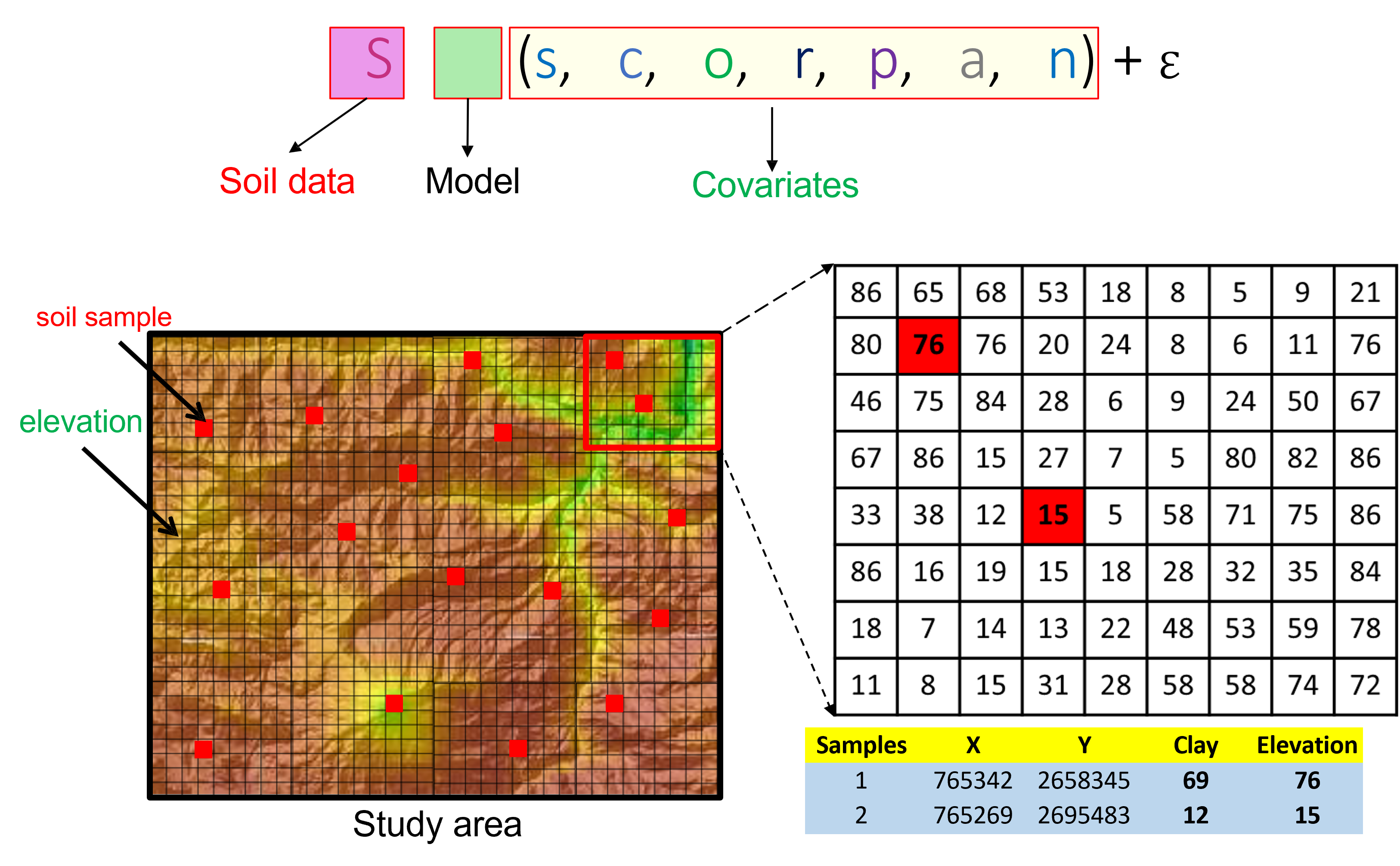
Figure 6.1: SCORPAN and relation with digital mapping.

\(\\[0.25cm]\)

Once we have several observation of the covariates a trend can be observed between variable values an samples boservation. It can follow a positive correlation or not.

\(\\[0.25cm]\)

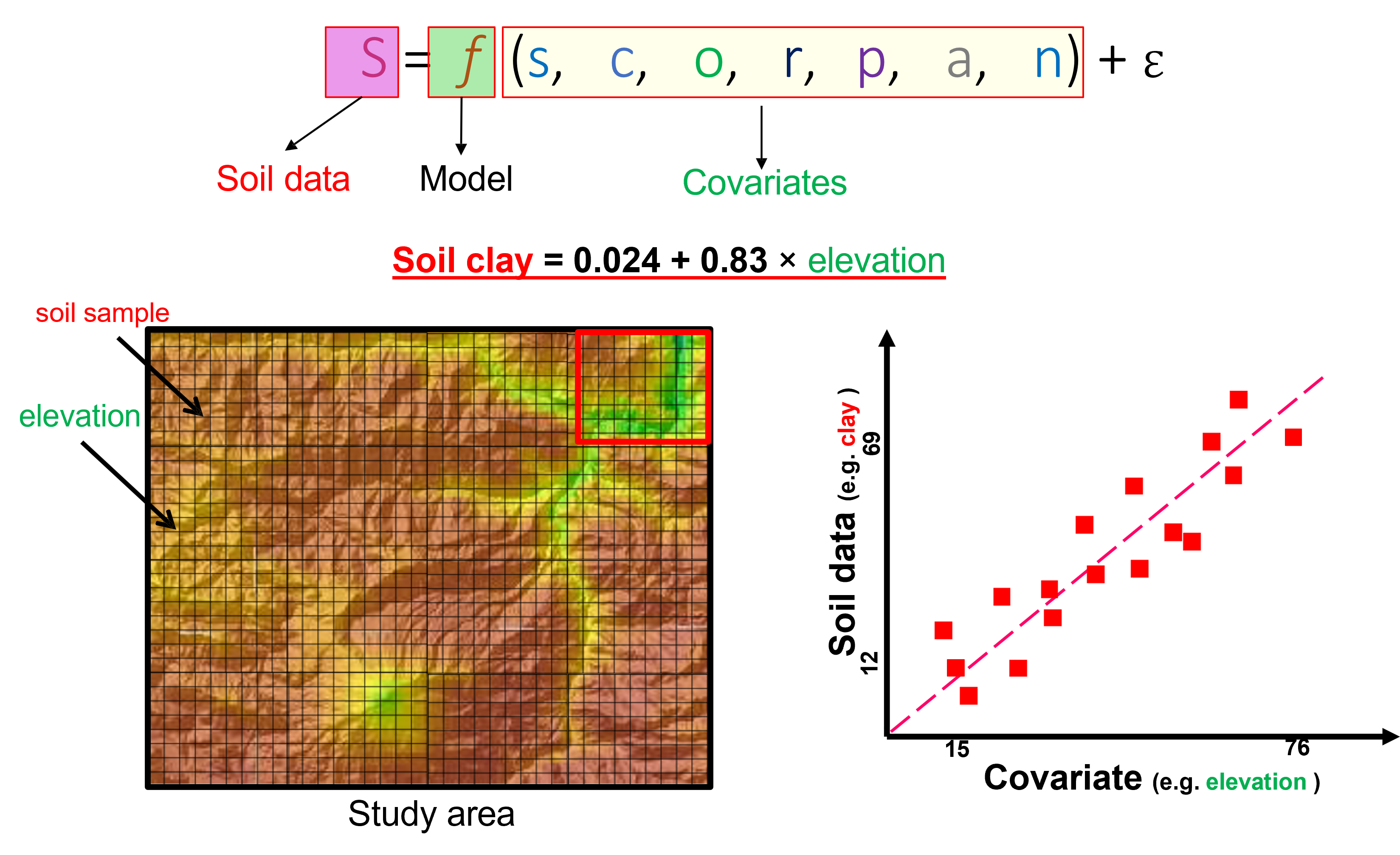
Figure 6.2: Covariates relation with soil observations.

6.2 Importing Covariates

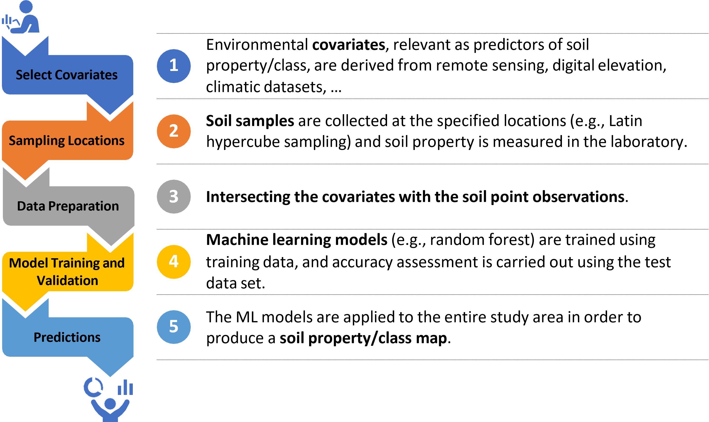
Figure 6.3: Digital soil mapping steps.

# empty memory and workspace
rm(list=ls())

# check directory
getwd()

## [1] "G:/OneDrive/Ecole/Cours/GEO-77/R_Introduction/Report"

# to install all required R packages
# install.packages("pacman")
library(pacman)

## Warning: le package 'pacman' a été compilé avec la version R 4.4.1

p_load("sp","raster","mapview","corrplot","randomForest","caret","rpart","rpart.plot")

# Import covariates (Remote Sensing, Terrain, Rainfall, NPP)
# import raster layers of covariates (Remote Sensing data)
blue = raster("./Data/DSM/RS/Blue.tif")
green = raster("./Data/DSM/RS/Green.tif")
red = raster("./Data/DSM/RS/Red.tif")
nir = raster("./Data/DSM/RS/Nir.tif")

6.2.1 Plot the Landsat layers

# calculate some Remote Sensing indices such as NDVI
ndvi = (nir - red) / (nir + red)

# make a stack layer from Remote Sensing data
landsat = stack(blue,green,red,nir,ndvi)

# set the names to the rasters in the stack file
names(landsat) <- c("blue","green","red","nir","ndvi")

# inspect the structure of stack layer
landsat

## class      : RasterStack 
## dimensions : 733, 716, 524828, 5  (nrow, ncol, ncell, nlayers)
## resolution : 500, 500  (x, y)
## extent     : 498000, 856000, 5235500, 5602000  (xmin, xmax, ymin, ymax)
## crs        : +proj=utm +zone=32 +datum=WGS84 +units=m +no_defs 
## names      :         blue,        green,          red,          nir,         ndvi 
## min values :   47.5000000,   92.0000000,   19.5000000,    6.0000000,   -0.6666667 
## max values : 9.383500e+03, 1.003950e+04, 1.027300e+04, 8.635500e+03, 8.870056e-01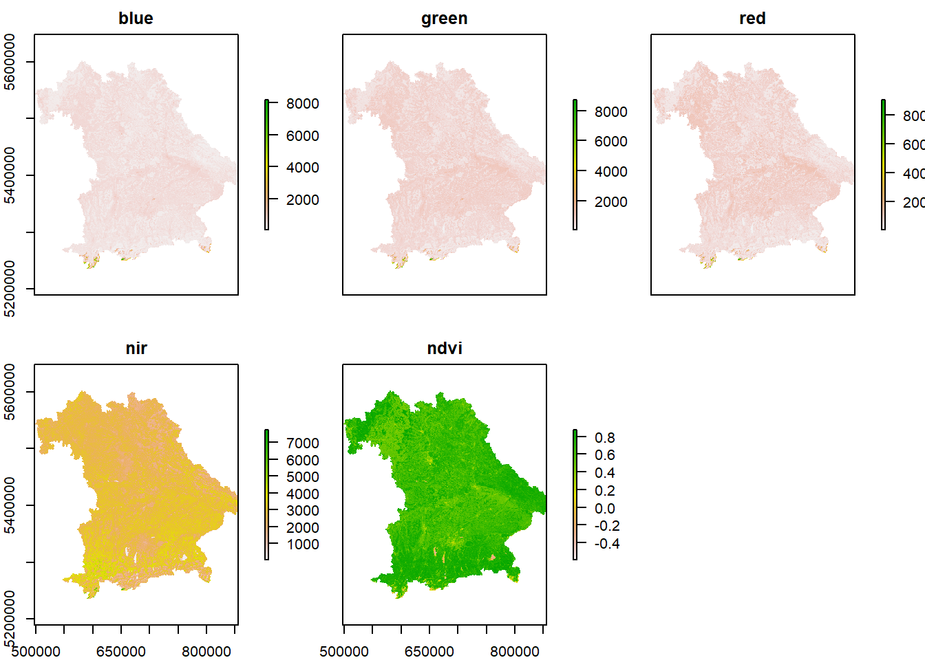

# plot the stack layers of Remote Sensing data
plot(landsat)

6.2.2 Stack and plot terrain variables

# import the terrain data using list.files command
dem_lst <- list.files("./Data/DSM/Terrain/", pattern="\\.sdat$", full.names = TRUE)

# inspect the structure of list
dem_lst

## [1] "./Data/DSM/Terrain/CNBL.sdat"  "./Data/DSM/Terrain/DEM.sdat"  
## [3] "./Data/DSM/Terrain/MCA.sdat"   "./Data/DSM/Terrain/Slope.sdat"
## [5] "./Data/DSM/Terrain/TWI.sdat"

# make a stack layer from terrain data 
terrain <- stack(dem_lst)

# plot the stack layers of terrain data
plot(terrain)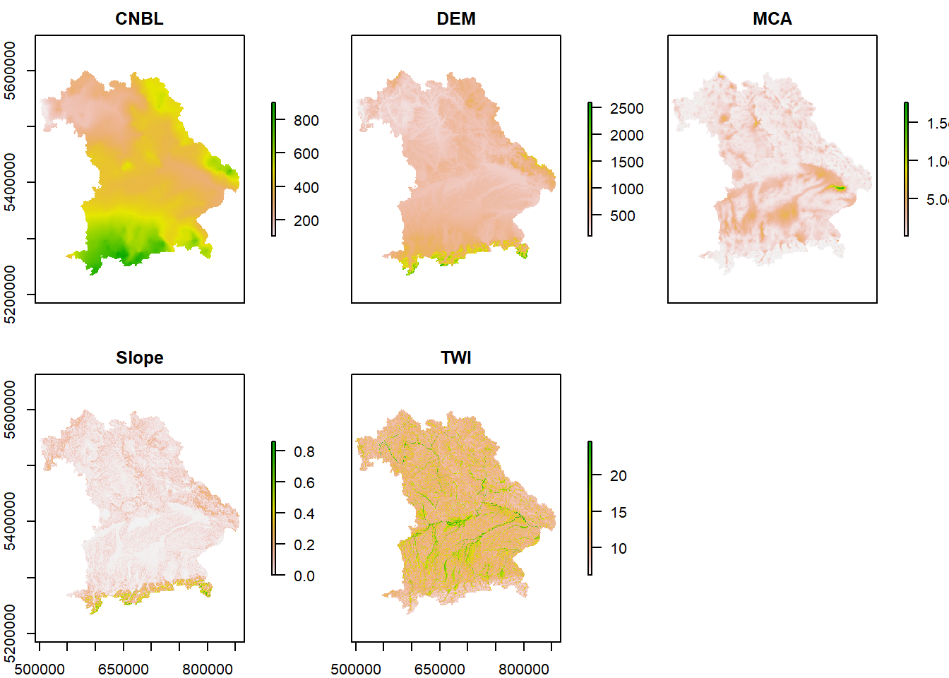

6.2.3 Plot and resample all covariates

# Re-sampling Remote Sensing data based on terrain data
RS_terrain = resample(landsat, terrain, method="bilinear")

# import mean annual rainfall (mm)
rain <- raster("./Data/DSM/Climate/rainfall.sdat")

# Re-sampling rainfall data based on terrain data
rain_terrain = resample(rain, terrain, method="bilinear")

# import Terra Net Primary Production kg*C/m^2
NPP <- raster("./Data/DSM/NPP/NPP.sdat")

# Re-sampling NPP based on terrain data
NPP_terrain = resample(NPP,terrain, method="bilinear")

# make a stack file from re-sampled remote sensing data, terrain data, rainfall, and NPP
covariates_stack = stack(terrain, RS_terrain, rain_terrain, NPP_terrain)

# inspect the structure of stack layer
names(covariates_stack)

##  [1] "CNBL"     "DEM"      "MCA"      "Slope"    "TWI"      "blue"    
##  [7] "green"    "red"      "nir"      "ndvi"     "rainfall" "NPP"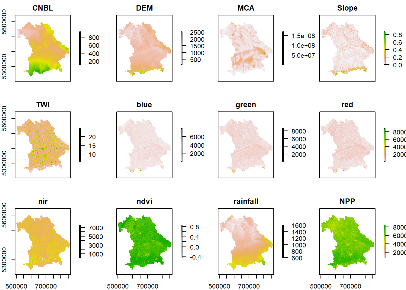

# plot the stack of covariates
plot(covariates_stack)

6.3 Importing study area and sampling locations

# import shape file of point data
point <- shapefile("./Data/DSM/Shapefile/points.shp")

# import shape file of Bavaria boundary
Bavaria = shapefile("./Data/DSM/Shapefile/Bavaria.shp")

# plot the point on the raster
plot(covariates_stack$DEM, main = "DEM", xlab = "Easting (m)", ylab = "Northing (m)")
plot(point,add =T, pch = 19)
plot(Bavaria, add =T)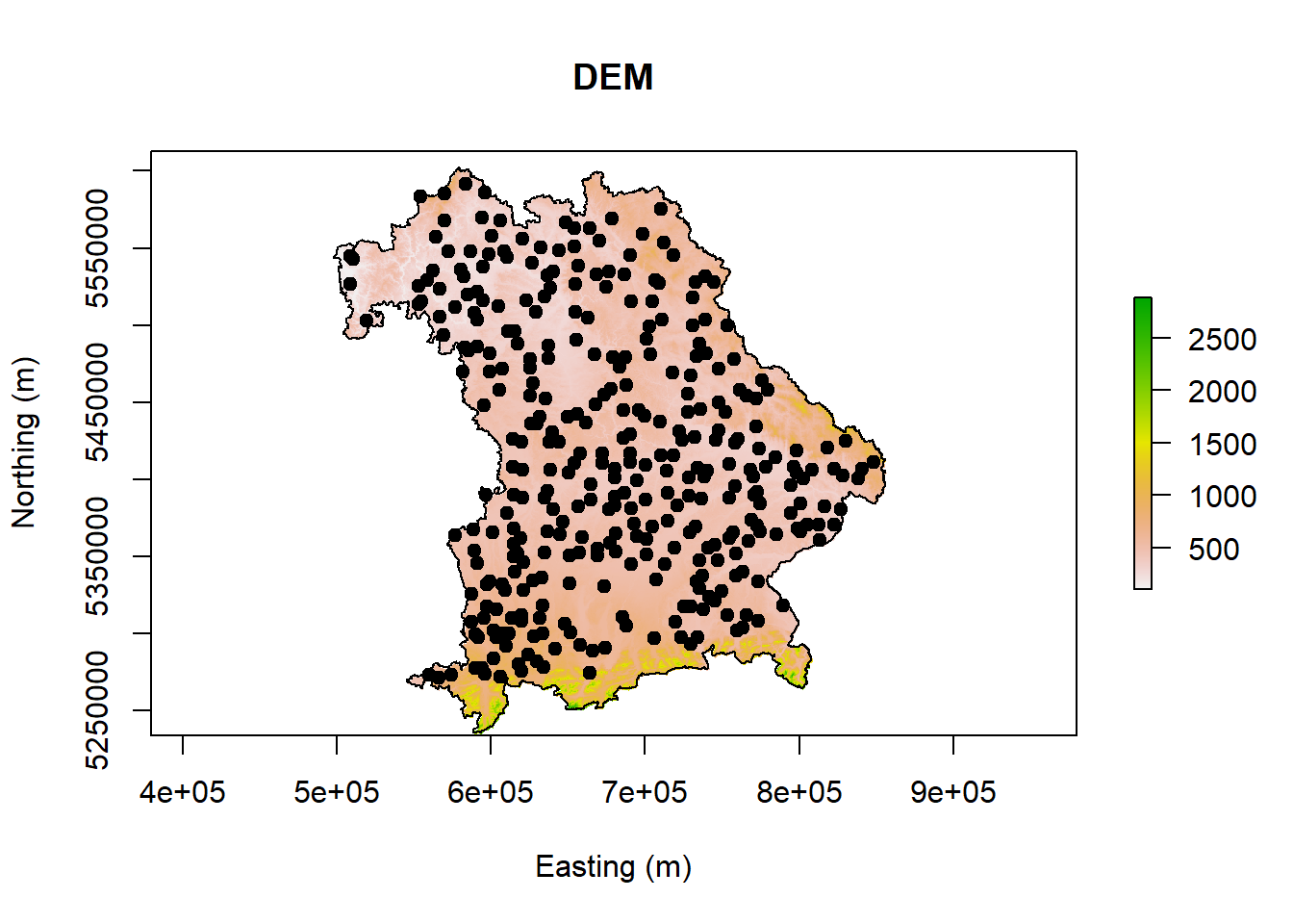

# plot an interactive map
mapview::mapview(point, zcol = "OC", at = c(0,5,10,15,20,25,30,35,200), legend = TRUE)

\(\\[0.15cm]\)

# inspect the point shape files
# types of the spatial data
class(point)

## [1] "SpatialPointsDataFrame"
## attr(,"package")
## [1] "sp"

# summary statistics of data
summary(point)

## Object of class SpatialPointsDataFrame
## Coordinates:
##         min       max
## x  508615.3  848381.1
## y 5271503.2 5591741.8
## Is projected: TRUE 
## proj4string :
## [+proj=utm +zone=32 +datum=WGS84 +units=m +no_defs]
## Number of points: 346
## Data attributes:
##        x                y                 pH              OC        
##  Min.   :508615   Min.   :5271503   Min.   :3.810   Min.   :  6.00  
##  1st Qu.:617164   1st Qu.:5352240   1st Qu.:6.162   1st Qu.: 14.50  
##  Median :672285   Median :5406629   Median :6.850   Median : 21.00  
##  Mean   :676277   Mean   :5416121   Mean   :6.738   Mean   : 28.35  
##  3rd Qu.:733674   3rd Qu.:5485267   3rd Qu.:7.380   3rd Qu.: 33.05  
##  Max.   :848381   Max.   :5591742   Max.   :8.140   Max.   :251.30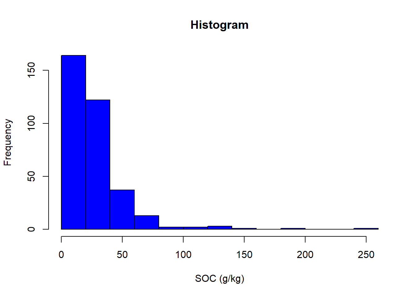

# histogram of SOC
hist(point$OC,col ="blue", xlab= "SOC (g/kg)", main="Histogram")

6.4 Extract the raster values at point locations

# extract covariate values at each point of observation 
cov = extract(covariates_stack, point, method='bilinear', df=TRUE)

# inspect the data.frame of cov
str(cov)

## 'data.frame':    346 obs. of  13 variables:
##  $ ID      : num  1 2 3 4 5 6 7 8 9 10 ...
##  $ CNBL    : num  398 431 587 408 535 ...
##  $ DEM     : num  426 493 600 474 544 ...
##  $ MCA     : num  6744760 14292214 4667933 5777121 14213043 ...
##  $ Slope   : num  0.0465 0.0149 0.026 0.0228 0.016 ...
##  $ TWI     : num  10.5 11.1 13.2 11.3 12 ...
##  $ blue    : num  236 401 374 375 411 ...
##  $ green   : num  403 698 599 670 680 ...
##  $ red     : num  273 680 537 586 544 ...
##  $ nir     : num  2561 3008 2808 3300 3390 ...
##  $ ndvi    : num  0.811 0.632 0.663 0.699 0.725 ...
##  $ rainfall: num  1105 1039 1105 964 1051 ...
##  $ NPP     : num  7384 6576 6772 6682 6919 ...

# combining covariates and soil properties
cov_soil = cbind(cov[,-1], OC=point$OC)
  
# inspect the data.frame of cov_soil
str(cov_soil)

## 'data.frame':    346 obs. of  13 variables:
##  $ CNBL    : num  398 431 587 408 535 ...
##  $ DEM     : num  426 493 600 474 544 ...
##  $ MCA     : num  6744760 14292214 4667933 5777121 14213043 ...
##  $ Slope   : num  0.0465 0.0149 0.026 0.0228 0.016 ...
##  $ TWI     : num  10.5 11.1 13.2 11.3 12 ...
##  $ blue    : num  236 401 374 375 411 ...
##  $ green   : num  403 698 599 670 680 ...
##  $ red     : num  273 680 537 586 544 ...
##  $ nir     : num  2561 3008 2808 3300 3390 ...
##  $ ndvi    : num  0.811 0.632 0.663 0.699 0.725 ...
##  $ rainfall: num  1105 1039 1105 964 1051 ...
##  $ NPP     : num  7384 6576 6772 6682 6919 ...
##  $ OC      : num  17.8 18 27.7 12.5 31.5 ...

# check the correlation covariates and OC
corrplot.mixed(cor(cov_soil), lower.col = "black", number.cex = .7)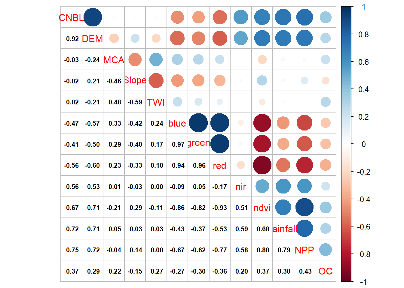

6.5 Prepare the data set before machine learning training

createDataPartition command to divide the data set into a p = split. It will create an index from which you will need to select the row belonging or not to the value.

set.seed allow you to create a specific randomness. Useful to reproduce an experiment.

# remove na values
cov_soil <- cov_soil[complete.cases(cov_soil),]

# remove high values of oc
cov_soil <- cov_soil[cov_soil$OC<78,]

# check number of rows
nrow(cov_soil)

## [1] 336

# check number of column 
ncol(cov_soil)

## [1] 13

# split the data to training (80%) and testing (20%) sets
set.seed(1234)
trainIndex <- createDataPartition(cov_soil$OC, 
                                  p = 0.8, list = FALSE, times = 1)

# subset the datasets
cov_soil_Train <- cov_soil[ trainIndex,]
cov_soil_Test  <- cov_soil[-trainIndex,]

# inspect the two datasets
str(cov_soil_Train)

## 'data.frame':    271 obs. of  13 variables:
##  $ CNBL    : num  431 587 535 414 403 ...
##  $ DEM     : num  493 600 544 466 408 ...
##  $ MCA     : num  14292214 4667933 14213043 18620790 22964809 ...
##  $ Slope   : num  0.01492 0.02598 0.01596 0.00466 0.00203 ...
##  $ TWI     : num  11.1 13.2 12 13 14.1 ...
##  $ blue    : num  401 374 411 472 489 ...
##  $ green   : num  698 599 680 810 806 ...
##  $ red     : num  680 537 544 783 797 ...
##  $ nir     : num  3008 2808 3390 3573 3300 ...
##  $ ndvi    : num  0.632 0.663 0.725 0.64 0.611 ...
##  $ rainfall: num  1039 1105 1051 984 931 ...
##  $ NPP     : num  6576 6772 6919 6549 6491 ...
##  $ OC      : num  18 27.7 31.5 12.4 17 72.8 15.2 30.7 17.4 20.2 ...

str(cov_soil_Test)

## 'data.frame':    65 obs. of  13 variables:
##  $ CNBL    : num  398 408 420 422 485 ...
##  $ DEM     : num  426 474 485 502 496 ...
##  $ MCA     : num  6744760 5777121 21438967 7046277 11136973 ...
##  $ Slope   : num  0.0465 0.0228 0.0103 0.0194 0.0192 ...
##  $ TWI     : num  10.5 11.3 11.3 10.4 14.1 ...
##  $ blue    : num  236 375 421 317 353 ...
##  $ green   : num  403 670 742 580 613 ...
##  $ red     : num  273 586 690 512 482 ...
##  $ nir     : num  2561 3300 3420 2784 3538 ...
##  $ ndvi    : num  0.811 0.699 0.666 0.693 0.758 ...
##  $ rainfall: num  1105 964 983 928 972 ...
##  $ NPP     : num  7384 6682 6859 6529 7115 ...
##  $ OC      : num  17.8 12.5 36.1 19.1 57.1 41.1 15 20.1 14.9 37.7 ...

6.6 Train the linear regression

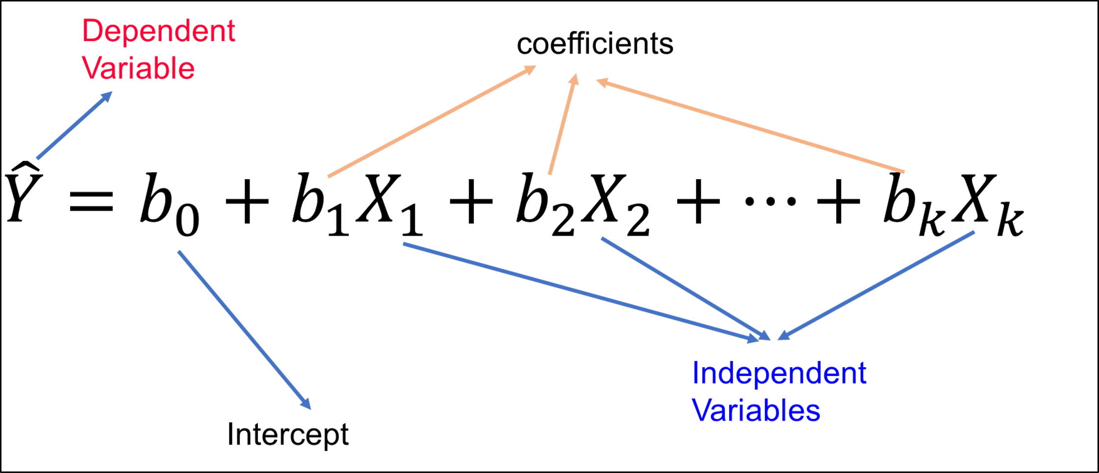
Figure 6.4: Linear regression schema.

lm(y ~ X, data = df) create a linear regression between y variables and X predictors (several columns) from the chosen data frame df. predict(model, test) predict the test values based on the train model. They need to have the same format (ncol, and colnames) as the training data.

# fit a linear regression on training set
set.seed(1234)
linear_fit <- lm(OC ~ CNBL+DEM+MCA+Slope+TWI+blue+green+red+nir+ndvi+rainfall+NPP, 
                 data=cov_soil_Train)

# look at the summary of linear model
summary(linear_fit)

## 
## Call:
## lm(formula = OC ~ CNBL + DEM + MCA + Slope + TWI + blue + green + 
##     red + nir + ndvi + rainfall + NPP, data = cov_soil_Train)
## 
## Residuals:
##     Min      1Q  Median      3Q     Max 
## -22.735  -7.836  -1.557   6.239  49.203 
## 
## Coefficients:
##               Estimate Std. Error t value Pr(>|t|)    
## (Intercept)  1.693e+02  5.694e+01   2.973 0.003225 ** 
## CNBL        -2.573e-02  2.026e-02  -1.270 0.205214    
## DEM          5.678e-02  1.928e-02   2.945 0.003526 ** 
## MCA          2.969e-07  8.091e-08   3.670 0.000295 ***
## Slope       -7.782e+01  4.139e+01  -1.880 0.061228 .  
## TWI          1.317e+00  3.987e-01   3.305 0.001085 ** 
## blue         7.050e-02  4.455e-02   1.583 0.114753    
## green       -3.596e-02  5.618e-02  -0.640 0.522727    
## red         -1.473e-01  3.888e-02  -3.790 0.000188 ***
## nir          2.749e-02  8.490e-03   3.237 0.001365 ** 
## ndvi        -2.306e+02  8.539e+01  -2.701 0.007369 ** 
## rainfall    -2.693e-02  1.032e-02  -2.611 0.009567 ** 
## NPP          5.853e-04  3.201e-03   0.183 0.855045    
## ---
## Signif. codes:  0 '***' 0.001 '**' 0.01 '*' 0.05 '.' 0.1 ' ' 1
## 
## Residual standard error: 11.51 on 258 degrees of freedom
## Multiple R-squared:  0.443,  Adjusted R-squared:  0.4171 
## F-statistic:  17.1 on 12 and 258 DF,  p-value: < 2.2e-16

# apply the linear model on testing data
OC_linear_Pred <- predict(linear_fit, cov_soil_Test)  

# check the plot actual and predicted OC values
plot(cov_soil_Test$OC, OC_linear_Pred, main="Linear model", 
     col="blue",xlab="Actual OC", ylab="Predicted OC", 
     xlim=c(0,100),ylim=c(0,100))
# Create a line of 1/1 showing the "perfect" prediction rate
abline(coef = c(0,1),  col="red" )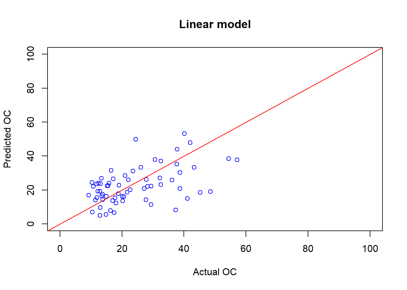

# calculate correlation
cor_linear <- cor(cov_soil_Test$OC, OC_linear_Pred)
cor_linear

## [1] 0.4996546

# calculate RMSE
RMSE_linear <- sqrt(mean((cov_soil_Test$OC - OC_linear_Pred)^2))
RMSE_linear

## [1] 11.30482

6.7 Train the decision tree

Decision tree schema [@alpaydin_introduction_2014].

Figure 6.5: Decision tree schema (Alpaydin 2014).

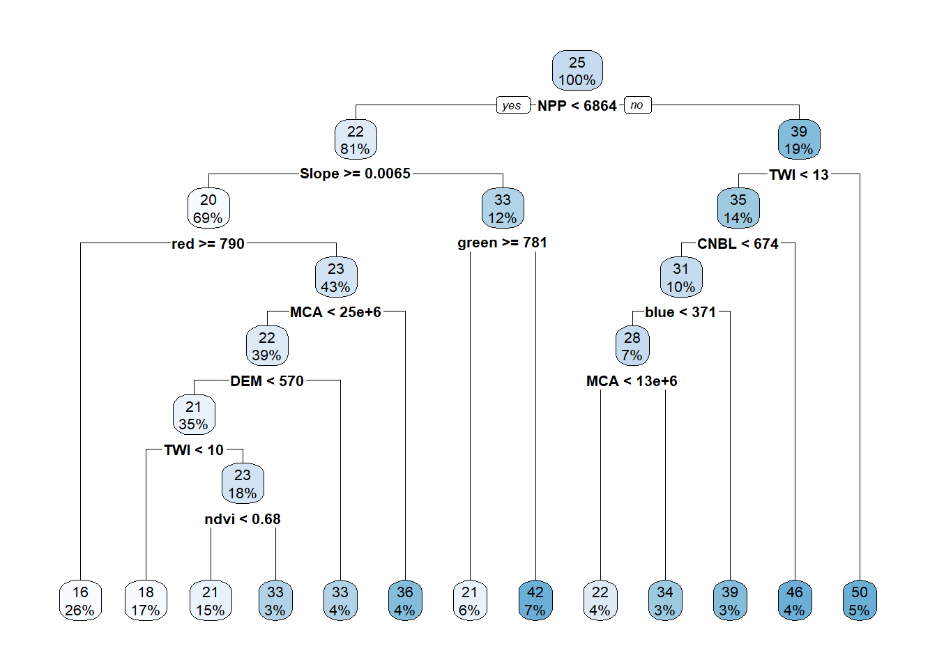
rpart(y ~ X, method = "", data = df) create a decision tree for the y variables and X predictors (several columns) from the chosen data frame df. The method parameter is by default “anova” but it can be change to “poisson” in case of discrete values. For classification problems the method can be set to “class”.

# fit decision tree model on training set
set.seed(1234)
tree_fit <- rpart(OC ~ CNBL+DEM+MCA+Slope+TWI+blue+green+red+nir+ndvi+rainfall+NPP,
                  method="anova", data=cov_soil_Train)

# display the results of decision tree
printcp(tree_fit)

## 
## Regression tree:
## rpart(formula = OC ~ CNBL + DEM + MCA + Slope + TWI + blue + 
##     green + red + nir + ndvi + rainfall + NPP, data = cov_soil_Train, 
##     method = "anova")
## 
## Variables actually used in tree construction:
##  [1] blue  CNBL  DEM   green MCA   ndvi  NPP   red   Slope TWI  
## 
## Root node error: 61351/271 = 226.39
## 
## n= 271 
## 
##          CP nsplit rel error  xerror     xstd
## 1  0.189128      0   1.00000 1.01112 0.104709
## 2  0.068565      1   0.81087 0.84893 0.097943
## 3  0.061621      2   0.74231 0.83187 0.096378
## 4  0.043476      3   0.68069 0.81398 0.094965
## 5  0.034078      4   0.63721 0.80606 0.095067
## 6  0.033352      5   0.60313 0.80303 0.094535
## 7  0.030887      6   0.56978 0.80303 0.094535
## 8  0.025692      7   0.53889 0.84399 0.099558
## 9  0.011202      8   0.51320 0.79923 0.091556
## 10 0.010799     10   0.49080 0.76902 0.083771
## 11 0.010465     11   0.48000 0.76902 0.083771
## 12 0.010000     12   0.46953 0.76559 0.083593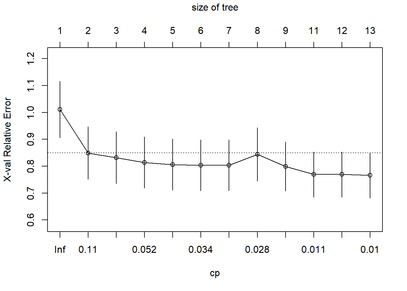

# visualize cross-validation results
plotcp(tree_fit)

# visualize the tree
rpart.plot(tree_fit)

# apply the tree model on testing data
OC_tree_Pred <- predict(tree_fit, cov_soil_Test)  

# check the plot actual and predicted OC values
plot(cov_soil_Test$OC, OC_tree_Pred, main="Tree model", 
     col="blue",xlab="Actual OC", ylab="Predicted OC", xlim=c(0,100),ylim=c(0,100))
abline(coef = c(0,1),  col="red" )

# calculate correlation
cor_tree <- cor(cov_soil_Test$OC, OC_tree_Pred)
cor_tree

## [1] 0.4036307

# calculate RMSE
RMSE_tree <- sqrt(mean((cov_soil_Test$OC - OC_tree_Pred)^2))
RMSE_tree

## [1] 12.02823

6.8 Train the Random forest

The random forest will produce several single decision trees and aggregate the results.

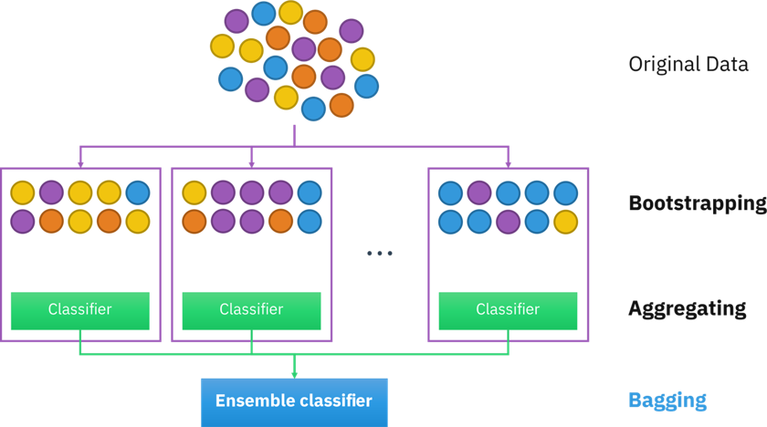
Figure 6.6: Random forest model.

randomForest(y ~ X, data = df) create a decision y variables and X predictors (several columns) from the chosen data frame df.

# fit random forest model on training set
set.seed(1234)
rf_fit <- randomForest(OC ~ CNBL+DEM+MCA+Slope+TWI+blue+green+red+nir+ndvi+rainfall+NPP, 
                       data=cov_soil_Train, ntree=500, do.trace = 25)

##      |      Out-of-bag   |
## Tree |      MSE  %Var(y) |
##   25 |    149.4    65.98 |
##   50 |    145.5    64.25 |
##   75 |    143.2    63.27 |
##  100 |    146.4    64.68 |
##  125 |    146.4    64.67 |
##  150 |    144.8    63.97 |
##  175 |    143.9    63.58 |
##  200 |    143.4    63.34 |
##  225 |    143.3    63.29 |
##  250 |    143.6    63.44 |
##  275 |      144    63.61 |
##  300 |    144.1    63.67 |
##  325 |    143.7    63.49 |
##  350 |    143.7    63.48 |
##  375 |    143.5    63.40 |
##  400 |    143.2    63.26 |
##  425 |      143    63.17 |
##  450 |    142.9    63.14 |
##  475 |      143    63.15 |
##  500 |    142.9    63.12 |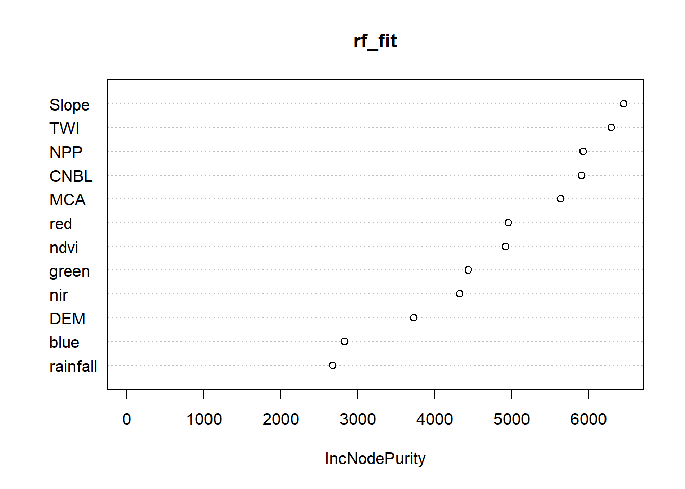

# visualize the importance of random forest
varImpPlot(rf_fit)

# apply the random forest model on testing data
OC_rf_Pred <- predict(rf_fit, cov_soil_Test)  

# check the plot actual and predicted OC values
plot(cov_soil_Test$OC, OC_rf_Pred, main="Tree model", 
     col="blue",xlab="Actual OC", ylab="Predicted OC", xlim=c(0,100),ylim=c(0,100))
abline(coef = c(0,1),  col="red" )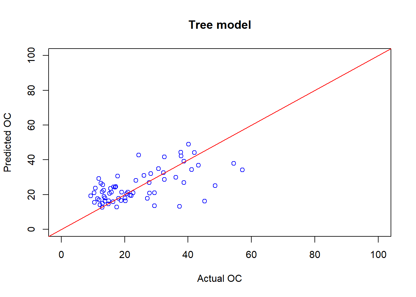

# calculate correlation
cor_rf <- cor(cov_soil_Test$OC, OC_rf_Pred)
cor_rf

## [1] 0.6036493

# calculate RMSE
RMSE_rf <- sqrt(mean((cov_soil_Test$OC - OC_rf_Pred)^2))
RMSE_rf

## [1] 9.617122

6.9 Comparing the results

We have to compare the different results of the models with RMSE and R² values.

# check the accuracy of three models
RMSE_models <- c(Linear=RMSE_linear,Tree=RMSE_tree,RF=RMSE_rf)
cor_models <- c(Linear=cor_linear,Tree=cor_tree,RF=cor_rf)

# plot the final results
par(mfrow=c(1,2))
barplot(RMSE_models, main="RMSE",col=c("red","blue","green"))
barplot(cor_models, main="Correlation",col=c("red","blue","green"))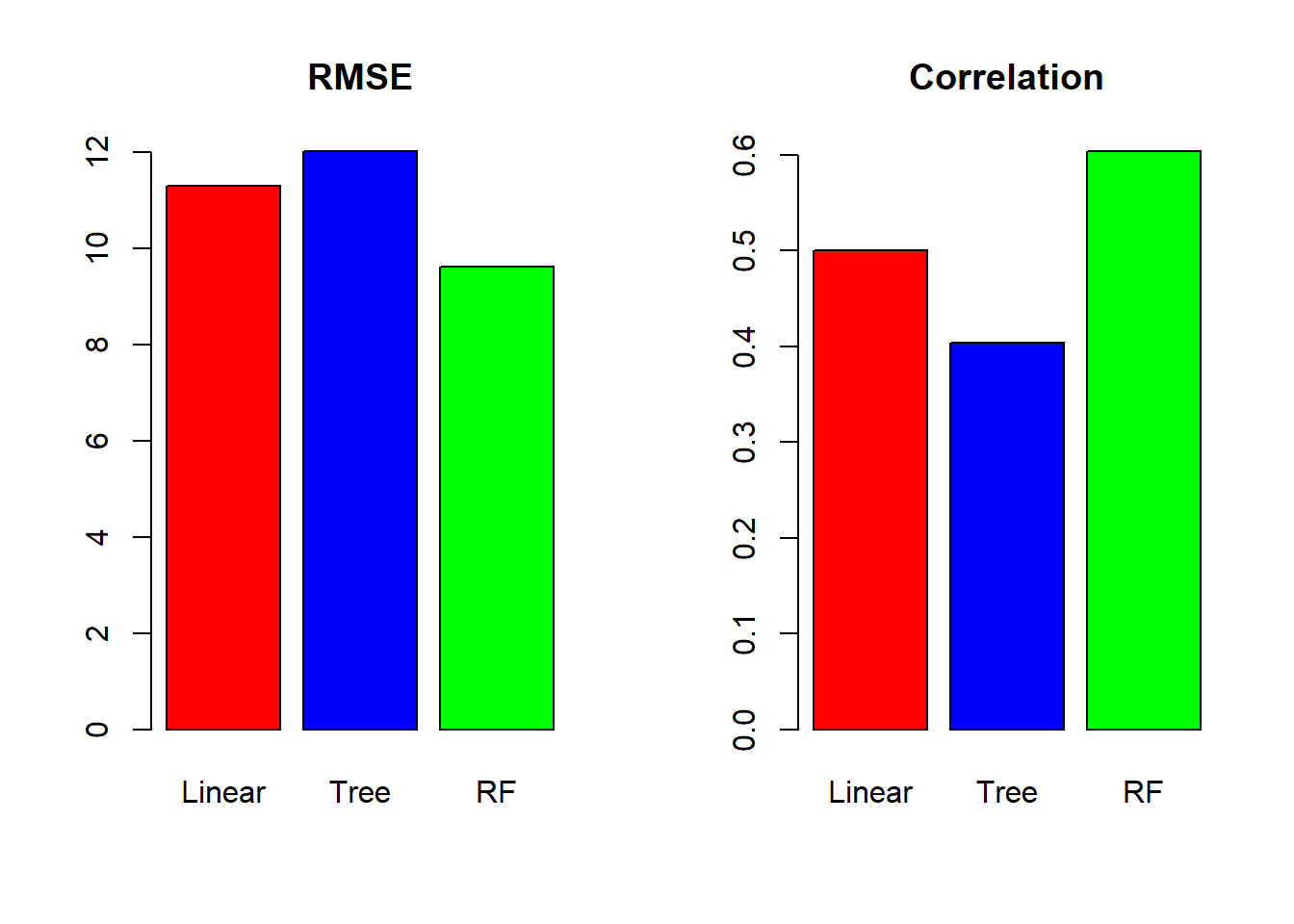

par(mfrow=c(1,1))

6.10 Create the prediction map

We are choosing the model with the best performances (RF). When predicting you do not need to set a seed.

# apply the best model on the stack layer
map_rf <- raster::predict(covariates_stack, rf_fit)

# plot the final map
spplot(map_rf, main="SOC map based on RF model")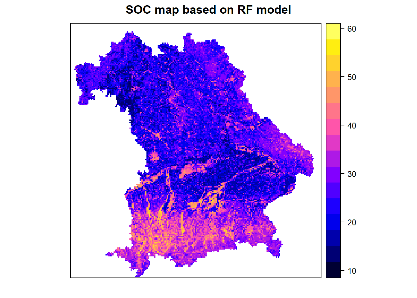

# plot an interactive map
mapview::mapview(map_rf)

6.11 Tuning the models

A model can be improved in many ways, but if you cannot obtain better training data or covariates, tuning the model is always a good option. By tuning the model, you will choose the best parameters for your dataset. Careful, however, not to overfit your model specifically to your data, in which case it could not be reusable afterwards.

The caret package is often used because it allows the deployment of a variety of machine learning commands.

6.11.1 Setting the general training parameters

To have a better model, you can create a cross-validation. It will take a small set of your data every time and use it as a testing set while using the remaining part. To create a cross-validation, you need to set the trainControl(method = "cv", number = x) parameter before running your model. X will represent the number of folds you want to perform.

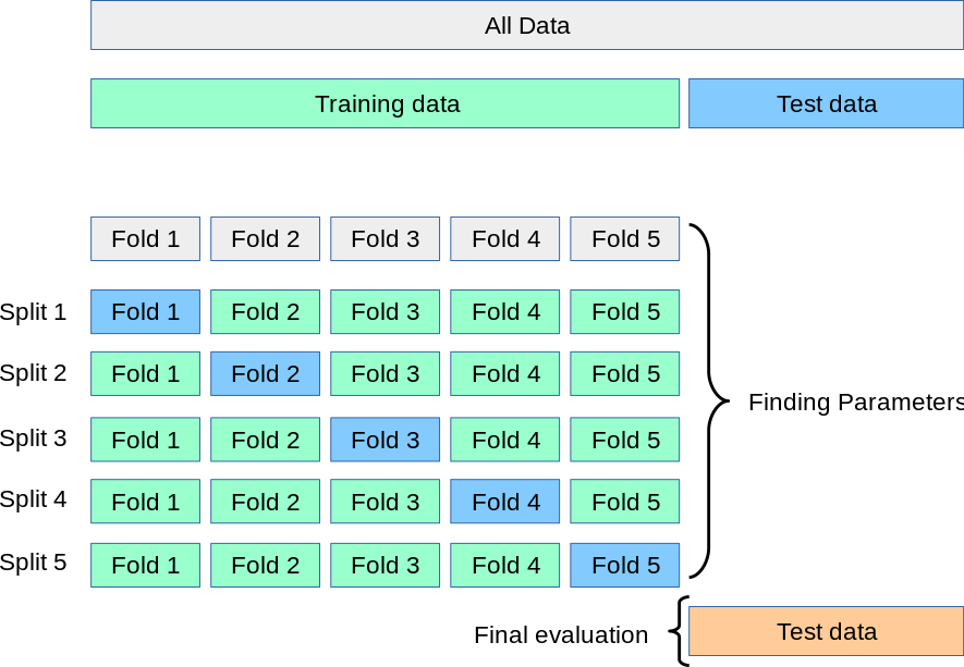
Figure 6.7: Cross validation fold schema.

Once the train control is set, you can create the training of the function with train(y ~ X, data =, method = "", trControl =, tuneGrid/tuneLength =, control =:

y will be the column name of the data you want to predict, and X will be the predictors (you can replace it with a .). The data is your training df.
method = "" is the model you want to chose. You can look to all caret package model on the webpage https://topepo.github.io/caret/available-models.html.
trControl = correspond to the trainControl() parameters we set earlier. -tuneGrid = is the tuning parameters of your model. You create a matrix of your tuning values with expand.grid function. For each model, the tuning variables have specific names. You can also use tuneLength, which randomly creates a grid of the number you set root square, the number of tuning parameters for this model (not recommended). You can also set a sequence of several numbers in your grid.
control an additional command for extra control parameters.

#First control parameters
ctrl1 <- trainControl(method = "cv", number = 5)
set.seed(1234)
tree_fit1 <- train(OC ~ CNBL+DEM+MCA+Slope+TWI+blue+green+red+nir+ndvi+rainfall+NPP,
                   data = cov_soil_Train,
                   method = "rpart",
                   trControl = ctrl1)


# display the results of decision tree
tree_fit1

## CART 
## 
## 271 samples
##  12 predictor
## 
## No pre-processing
## Resampling: Cross-Validated (5 fold) 
## Summary of sample sizes: 215, 217, 217, 218, 217 
## Resampling results across tuning parameters:
## 
##   cp          RMSE      Rsquared    MAE     
##   0.06162053  13.80990  0.19138312  10.31556
##   0.06856500  13.90378  0.18603785  10.39489
##   0.18912794  14.63942  0.09680234  11.41884
## 
## RMSE was used to select the optimal model using the smallest value.
## The final value used for the model was cp = 0.06162053.

cat( "Decision tree model 1 had", nrow(tree_fit1$resample), "Run in total \n")

## Decision tree model 1 had 5 Run in total

#Second control parameters
ctrl2 <- trainControl(method = "cv", number = 20)
set.seed(1234)
tree_fit2 <- train(OC ~ CNBL+DEM+MCA+Slope+TWI+blue+green+red+nir+ndvi+rainfall+NPP,
                   data = cov_soil_Train,
                   method = "rpart",
                   trControl = ctrl2)

# display the results of decision tree
tree_fit2

## CART 
## 
## 271 samples
##  12 predictor
## 
## No pre-processing
## Resampling: Cross-Validated (20 fold) 
## Summary of sample sizes: 257, 256, 258, 258, 257, 256, ... 
## Resampling results across tuning parameters:
## 
##   cp          RMSE      Rsquared    MAE     
##   0.06162053  13.77702  0.22658828  10.43208
##   0.06856500  14.07502  0.20270384  10.74035
##   0.18912794  14.85486  0.07527534  11.60622
## 
## RMSE was used to select the optimal model using the smallest value.
## The final value used for the model was cp = 0.06162053.

cat( "Decision tree model 2 had", nrow(tree_fit2$resample), "Run in total \n")

## Decision tree model 2 had 20 Run in total

You can also repeat the cross-validation several time with the method = "repeatedcv"

#Third control parameters
ctrl3 <- trainControl(method = "repeatedcv", number = 5, repeats = 3)
set.seed(1234)
tree_fit3 <- train(OC ~ CNBL+DEM+MCA+Slope+TWI+blue+green+red+nir+ndvi+rainfall+NPP,
                   data = cov_soil_Train,
                   method = "rpart",
                   trControl = ctrl3)


# display the results of decision tree
tree_fit3

## CART 
## 
## 271 samples
##  12 predictor
## 
## No pre-processing
## Resampling: Cross-Validated (5 fold, repeated 3 times) 
## Summary of sample sizes: 215, 217, 217, 218, 217, 215, ... 
## Resampling results across tuning parameters:
## 
##   cp          RMSE      Rsquared    MAE     
##   0.06162053  13.98031  0.18955436  10.46265
##   0.06856500  14.15751  0.17382230  10.58568
##   0.18912794  14.67725  0.09851222  11.38858
## 
## RMSE was used to select the optimal model using the smallest value.
## The final value used for the model was cp = 0.06162053.

cat( "Decision tree model 3 had", nrow(tree_fit3$resample), "Run in total \n")

## Decision tree model 3 had 15 Run in total

6.11.2 Decision tree model tuning

rpart.control() Function allows you to tune your decision tree model:

cp is the complexity parameter that will set pruning. The lowest the number sits, the more complex the tree becomes.
minsplit is the minimum number of observations needed for a split.
minbucket is the minimum number of observations in a leaf.
maxdepth is the maximum depth of the tree.

On the parameters of the decision tree, you can specify the tuneGrid parameter from the caret training with an expand.grid()

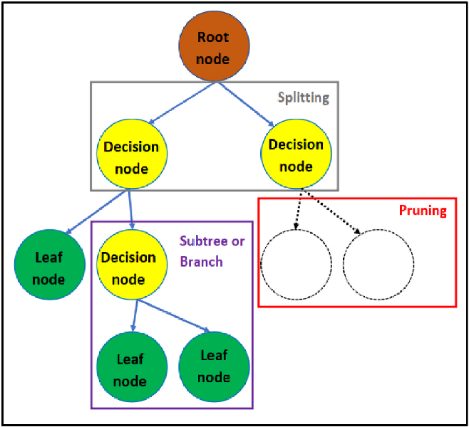
Figure 6.8: Decision tree parameters.

# Create a decision tree with simpler parameters
rpart_ctrl1 <- rpart.control(
  cp = 0.05,       # Complexity parameter 
  minsplit = 20,    # Minimum number of observations to split
  minbucket = 15,    # Minimum number of observations in any terminal node
  maxdepth = 4      # Maximum depth of the tree
)


set.seed(1234)
tree_fit4 <- rpart(OC ~ CNBL+DEM+MCA+Slope+TWI+blue+green+red+nir+ndvi+rainfall+NPP,
                  method="anova", data=cov_soil_Train, control = rpart_ctrl1)

# display the results of the more simple decision tree
printcp(tree_fit4)

## 
## Regression tree:
## rpart(formula = OC ~ CNBL + DEM + MCA + Slope + TWI + blue + 
##     green + red + nir + ndvi + rainfall + NPP, data = cov_soil_Train, 
##     method = "anova", control = rpart_ctrl1)
## 
## Variables actually used in tree construction:
## [1] green NPP   Slope
## 
## Root node error: 61351/271 = 226.39
## 
## n= 271 
## 
##         CP nsplit rel error  xerror     xstd
## 1 0.189128      0   1.00000 1.01112 0.104709
## 2 0.068565      1   0.81087 0.84893 0.097943
## 3 0.061621      2   0.74231 0.79133 0.094026
## 4 0.050000      3   0.68069 0.78313 0.093608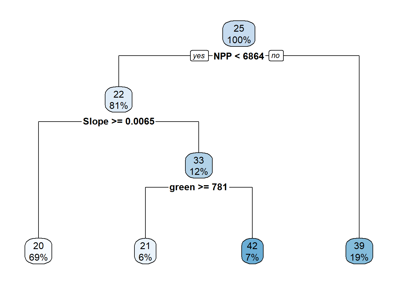

# visualize the more simple tree
rpart.plot(tree_fit4)

# Create a decision tree with more complex parameters
rpart_ctrl2 <- rpart.control(
  cp = 0.0005,       # Complexity parameter 
  minsplit = 10,    # Minimum number of observations to split
  minbucket = 5,    # Minimum number of observations in any terminal node
  maxdepth = 8      # Maximum depth of the tree
)


set.seed(1234)
tree_fit5 <- rpart(OC ~ CNBL+DEM+MCA+Slope+TWI+blue+green+red+nir+ndvi+rainfall+NPP,
                  method="anova", data=cov_soil_Train, control = rpart_ctrl2)

# display the results of the more simple decision tree
printcp(tree_fit5)

## 
## Regression tree:
## rpart(formula = OC ~ CNBL + DEM + MCA + Slope + TWI + blue + 
##     green + red + nir + ndvi + rainfall + NPP, data = cov_soil_Train, 
##     method = "anova", control = rpart_ctrl2)
## 
## Variables actually used in tree construction:
##  [1] blue     CNBL     DEM      green    MCA      ndvi     nir      NPP     
##  [9] rainfall red      Slope    TWI     
## 
## Root node error: 61351/271 = 226.39
## 
## n= 271 
## 
##           CP nsplit rel error  xerror     xstd
## 1  0.1891279      0   1.00000 1.01112 0.104709
## 2  0.0685650      1   0.81087 0.84893 0.097943
## 3  0.0616205      2   0.74231 0.83187 0.096378
## 4  0.0434759      3   0.68069 0.80149 0.094160
## 5  0.0345742      4   0.63721 0.82250 0.095723
## 6  0.0333516      6   0.56806 0.81490 0.096209
## 7  0.0256923      7   0.53471 0.85861 0.103798
## 8  0.0221136      8   0.50902 0.85129 0.103001
## 9  0.0184032      9   0.48690 0.86388 0.102180
## 10 0.0163354     10   0.46850 0.83239 0.099363
## 11 0.0163285     11   0.45217 0.84990 0.100276
## 12 0.0151540     12   0.43584 0.84632 0.099720
## 13 0.0134087     13   0.42068 0.84857 0.100390
## 14 0.0118905     14   0.40727 0.83985 0.099958
## 15 0.0098702     15   0.39538 0.89144 0.109507
## 16 0.0087546     18   0.36577 0.92894 0.116296
## 17 0.0071396     19   0.35702 0.92501 0.116260
## 18 0.0063750     20   0.34988 0.93275 0.115394
## 19 0.0057885     21   0.34350 0.93703 0.115343
## 20 0.0046200     22   0.33772 0.95163 0.115323
## 21 0.0036255     23   0.33310 0.96827 0.116000
## 22 0.0031440     25   0.32584 0.96285 0.113771
## 23 0.0027501     26   0.32270 0.96343 0.113770
## 24 0.0019185     27   0.31995 0.96954 0.113830
## 25 0.0010823     28   0.31803 0.96873 0.113780
## 26 0.0009681     29   0.31695 0.97503 0.114070
## 27 0.0005000     30   0.31598 0.97487 0.114053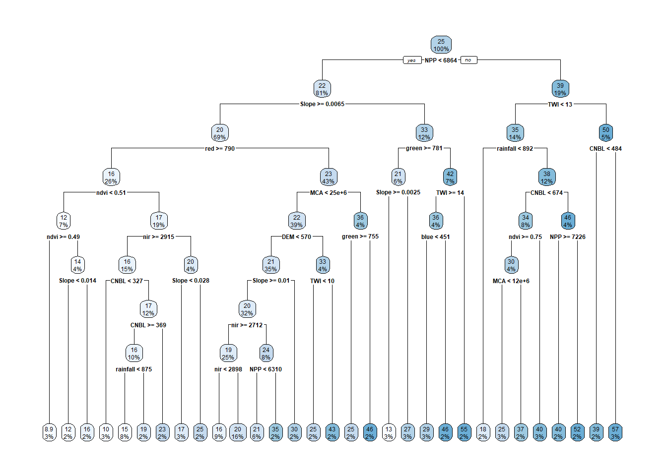

# visualize the more simple tree
rpart.plot(tree_fit5)

6.11.3 Random forest model tuning

For the random forest algorithm, you have two main tuning parameters:

ntree decides the number of decision trees to generate. By default, it is set at 500, which is a good number, but you can change it with the ntree = command line in the caret train function.
mtry is the number of variables selected for each split; the higher it is, the more complex your model becomes. In the caret train function, you specify with the trainGrid = parameter.

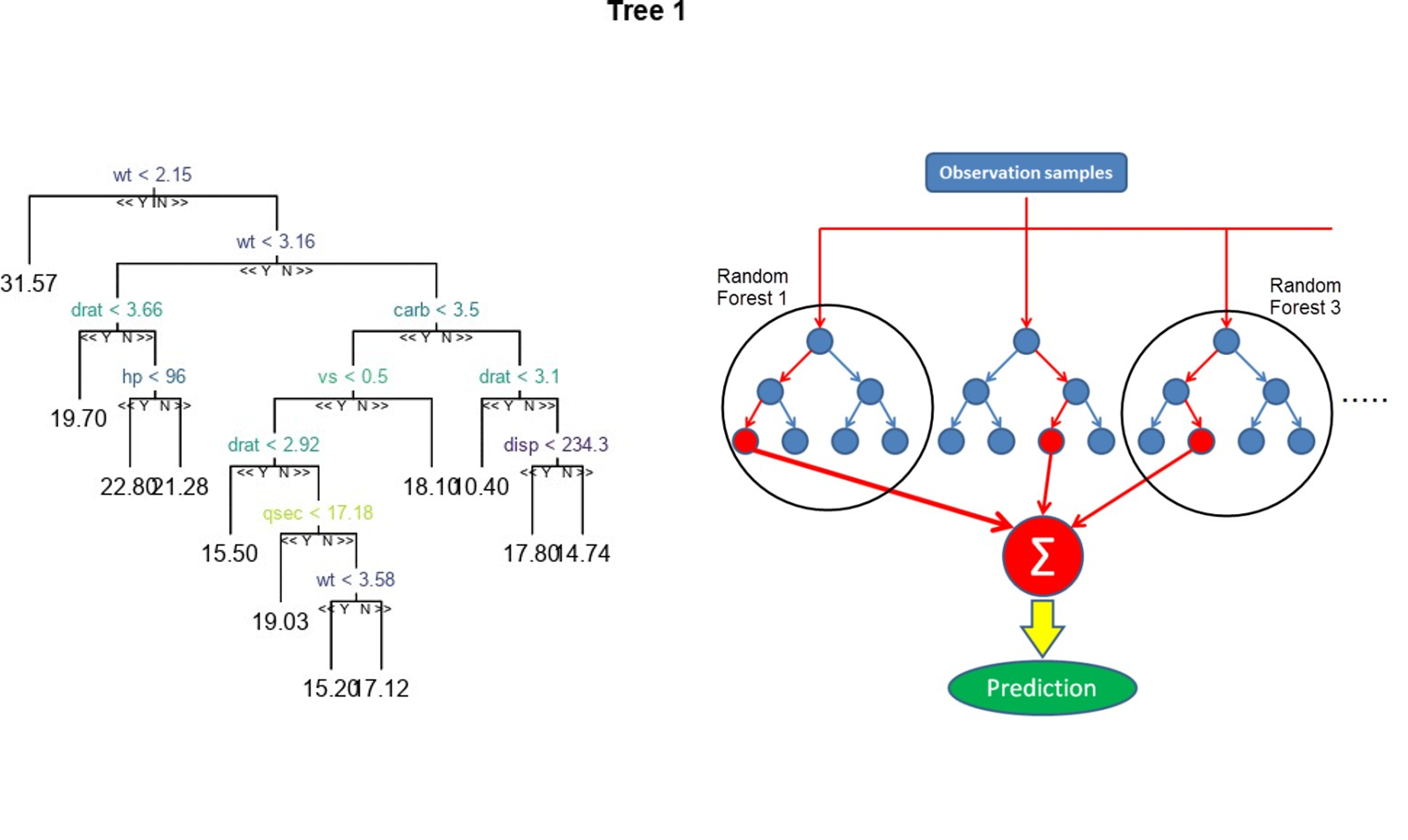
Figure 6.9: Random forest detailed schema.

# First RF tree with less complexity
ctrl <- trainControl(method = "cv", number = 10)

rfGrid1 <- expand.grid(.mtry = 3)

set.seed(1234)
rf_fit1 <- train(OC ~ CNBL+DEM+MCA+Slope+TWI+blue+green+red+nir+ndvi+rainfall+NPP,
                   data = cov_soil_Train,
                   method = "rf",
                   trControl = ctrl,
                   tuneGrid = rfGrid1,
                   ntree = 200)

rf_fit1$finalModel

## 
## Call:
##  randomForest(x = x, y = y, ntree = 200, mtry = param$mtry) 
##                Type of random forest: regression
##                      Number of trees: 200
## No. of variables tried at each split: 3
## 
##           Mean of squared residuals: 147.4249
##                     % Var explained: 34.88

rf_fit1$results

##   mtry     RMSE  Rsquared      MAE  RMSESD RsquaredSD    MAESD
## 1    3 11.67351 0.3984199 8.919224 2.01285  0.1343811 1.345439

# Second RF tree with more complexity
rfGrid2 <- expand.grid(.mtry = 6)

set.seed(1234)
rf_fit2 <- train(OC ~ CNBL+DEM+MCA+Slope+TWI+blue+green+red+nir+ndvi+rainfall+NPP,
                   data = cov_soil_Train,
                   method = "rf",
                   trControl = ctrl,
                   tuneGrid = rfGrid2,
                   ntree = 1000)

rf_fit2$finalModel

## 
## Call:
##  randomForest(x = x, y = y, ntree = 1000, mtry = param$mtry) 
##                Type of random forest: regression
##                      Number of trees: 1000
## No. of variables tried at each split: 6
## 
##           Mean of squared residuals: 144.8437
##                     % Var explained: 36.02

rf_fit2$results

##   mtry     RMSE  Rsquared      MAE   RMSESD RsquaredSD    MAESD
## 1    6 11.72908 0.3922939 8.954656 1.889745  0.1179939 1.255245

# Testing several tuning parameters at the same time
rfGrid3 <- expand.grid(.mtry = c(3:6))

set.seed(1234)
rf_fit3 <- train(OC ~ CNBL+DEM+MCA+Slope+TWI+blue+green+red+nir+ndvi+rainfall+NPP,
                   data = cov_soil_Train,
                   method = "rf",
                   trControl = ctrl,
                   tuneGrid = rfGrid3,
                   ntree = 500)

rf_fit3$finalModel

## 
## Call:
##  randomForest(x = x, y = y, ntree = 500, mtry = param$mtry) 
##                Type of random forest: regression
##                      Number of trees: 500
## No. of variables tried at each split: 4
## 
##           Mean of squared residuals: 143.2986
##                     % Var explained: 36.7

rf_fit3$results

##   mtry     RMSE  Rsquared      MAE   RMSESD RsquaredSD    MAESD
## 1    3 11.69037 0.3969708 8.892300 1.938197  0.1289380 1.268843
## 2    4 11.68114 0.3955169 8.896886 1.862187  0.1186351 1.237828
## 3    5 11.71240 0.3937666 8.912386 1.913175  0.1229028 1.264399
## 4    6 11.71687 0.3921174 8.908756 1.921134  0.1210158 1.230857

6.12 Variables importance

There are several ways of assessing the variable importance of the model and the node impurity. The ** Gini** index or Gini ratio provides a ranking of the attributes for splitting the data. It stores the sum of the squared probabilities of each class or value. it can be used for classification problems.

\(Gini = 1 - \sum(P_i)^2\)

\(i\) = 1 to the number of classes. \(P\) = probabilities of each class.

With 0, the Gini impurity index is at its lowest. It occurs only when all the elements of the split are from the same class/value.

With a caret model trained you can use the varImp function to see the Gini index of all variables.

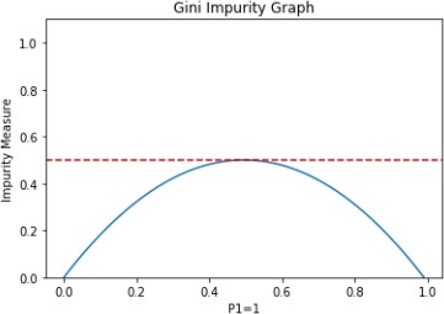
Figure 6.10: Gini impurity index.

\(\\[0.25cm]\)

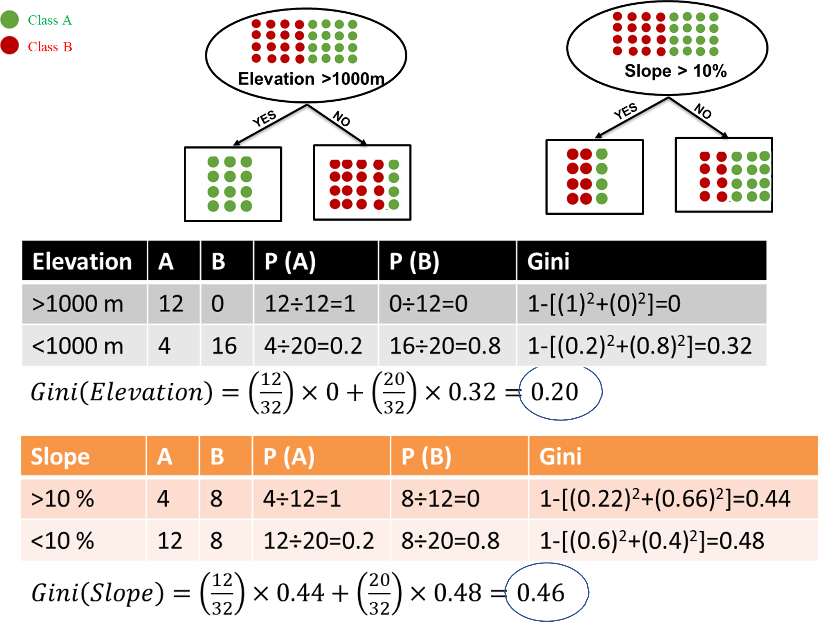
Figure 6.11: Gini formula example.

\(\\[0.2cm]\)

For regression problems MSE is a more adapted impurity measurement.

\(MSE = \frac{1}{n} \sum_{i=1}^{n}(Y_i - \hat{Y}_i)^2\)

\(n\) = the number of measurements. \(Y\) = the observed value. \(\hat{Y}\) = the predicted value

# Ploting variable importance

importance_rf <- varImp(rf_fit3)
importance_rf

## rf variable importance
## 
##          Overall
## Slope    100.000
## TWI       91.693
## NPP       86.851
## MCA       78.089
## CNBL      75.723
## ndvi      73.076
## red       57.213
## nir       45.278
## green     42.216
## DEM       30.440
## blue       8.825
## rainfall   0.000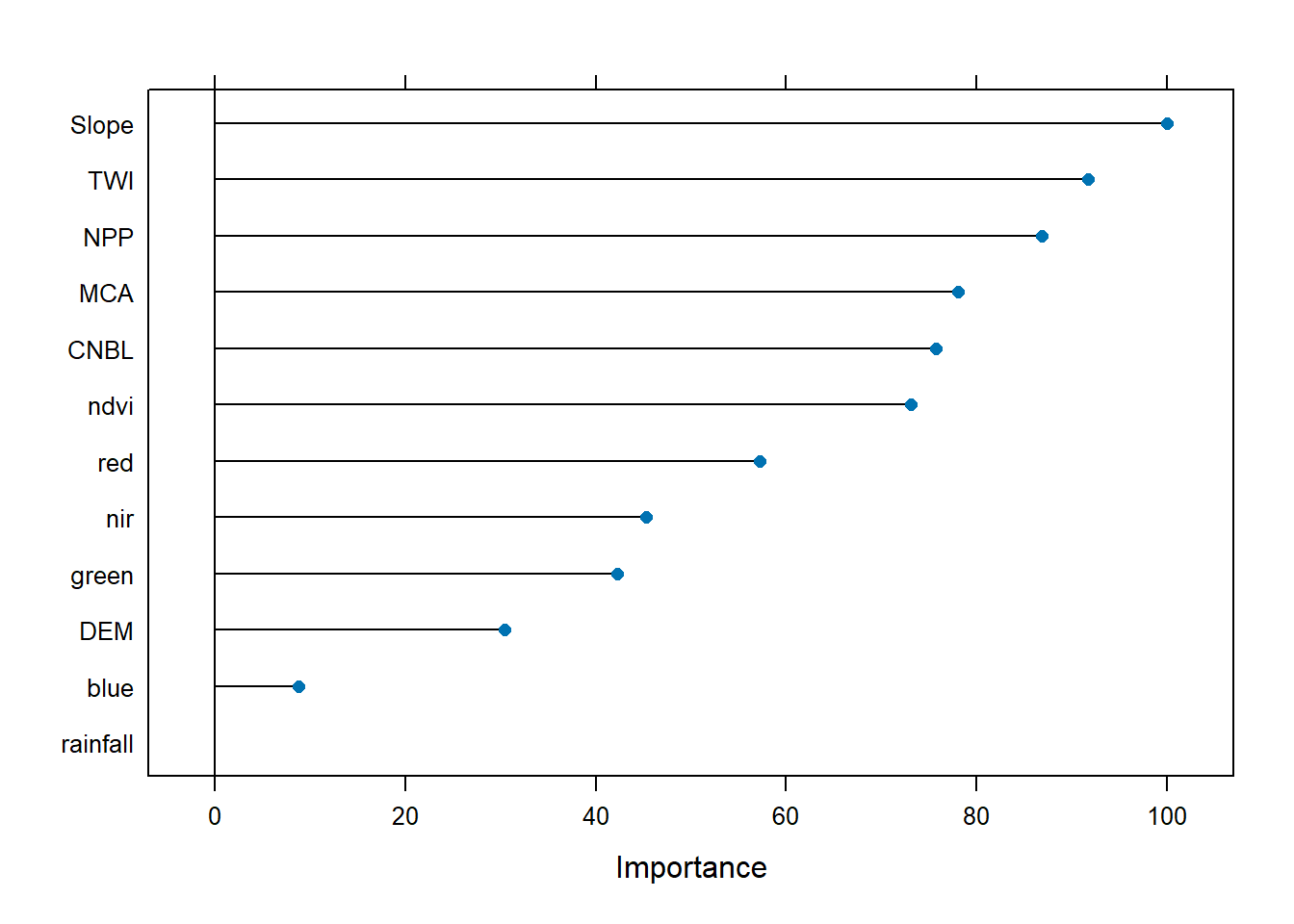

plot(importance_rf)

# More complex plot using ggplot function

# Set results in a df
importance_data <- as.data.frame(importance_rf$importance)
importance_data$Variable <- rownames(importance_data)

# Scaled it in percent and organising it in decreasing order
importance_data$Percentage <- importance_data$Overall / sum(importance_data$Overall) * 100
importance_data <- importance_data[order(importance_data$Percentage, decreasing = TRUE), ]


# Create the graph
importance_graph <- ggplot(importance_data, aes(x = reorder(Variable, Percentage), y = Percentage)) +
  geom_bar(stat = "identity", fill = "skyblue", color = "black", width = 0.7, alpha = 0.7) +
  coord_flip() +
  labs(
    title = "Importance of variables in percent",
    x = "Variable",
    y = "Importance (%)"
  ) +
  theme_classic() +
  theme(
    axis.text = element_text(size = 12, color = "black"),
    axis.title = element_text(size = 14, face = "bold"),
    plot.title = element_text(size = 16, face = "bold", hjust = 0.5)
  ) +
  geom_text(aes(label = round(Percentage, 1)), hjust = -0.2, color = "black", size = 4) +
  ylim(0, max(importance_data$Percentage) * 1.1)

importance_graph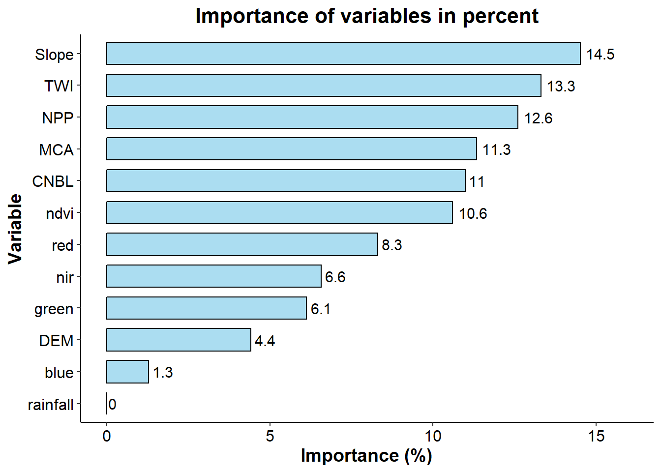

# Option to export the plot
#ggsave( "./Variables_importance_RF.pdf", importance_graph, width = 20, height = 13, units = "cm")

Alpaydin, Ethem. 2014. Introduction to Machine Learning. Third edition. Adaptive Computation and Machine Learning. Cambridge, Massachusetts: The MIT Press.

Giorgi, Federico M., Carmine Ceraolo, and Daniele Mercatelli. 2022. “The R Language: An Engine for Bioinformatics and Data Science.” Life 12 (5): 648. https://doi.org/10.3390/life12050648.

Ihaka, Ross, and Robert Gentleman. 1996. “R: A Language for Data Analysis and Graphics.” Journal of Computational and Graphical Statistics 5 (3): 299. https://doi.org/10.2307/1390807.

Long, J. D., and Paul Teetor. 2019. R Cookbook: Proven Recipes for Data Analysis, Statistics, and Graphics. Second edition. Sebastopol, CA: O’Reilly.

McBratney, A. B, M. L Mendonça Santos, and B Minasny. 2003. “On Digital Soil Mapping.” Geoderma 117 (1-2): 3–52. https://doi.org/10.1016/S0016-7061(03)00223-4.

Team, R Core, W. N. Venables, and D. M. Smith. 2022. An Introduction to R: A Programming Environment for Data Analysis and Graphics, Version 4.2.1. 4th ed.

Tippmann, Sylvia. 2015. “Programming Tools: Adventures with R.” Nature 517 (7532): 109–10. https://doi.org/10.1038/517109a.

References

Alpaydin, Ethem. 2014. Introduction to Machine Learning. Third edition. Adaptive Computation and Machine Learning. Cambridge, Massachusetts: The MIT Press.

McBratney, A. B, M. L Mendonça Santos, and B Minasny. 2003. “On Digital Soil Mapping.” Geoderma 117 (1-2): 3–52. https://doi.org/10.1016/S0016-7061(03)00223-4.