1 R Introduction Course
1.1 General introduction
1.1.1 Short history and philosophy of R
R is a free and open-source system developed at the beginning of the 1990s by Ross Ihaka and Robert Gentleman at Auckland University (1993). In 1996 they published the first paper on R language (Ihaka and Gentleman 1996) named: Ross Ihaka and Robert Gentleman. R:“A language for data analysis and graphics.” Journal of Computational and Graphical Statistics, 5(3):299–314, 1996, and in 1997 started the R Core Group/Team a team of statisticians and computer scientists. They released in 2000 the first public version of R (1.0.0). In addition to this, the Comprehensive R Archive Network or CRAN where the R code is stored, also hosted additional packages from users. On 03/10/2022 more than 20,000 packages were stored on the CRAN against 200 in 2003 and 9,000 in 2015 (Tippmann 2015).
Another important part of R is its free-user dimension. The development of this language was highly inspired by a previous language the S. Developed by John Chambers in the Nokia Bell Laboratory during the 1970s it was designed by and for data scientists and not programmers. The philosophy of freely accessible software for everyone quickly developed and can be described as :
“[We] wanted users to be able to begin in an interactive environment, where they did not consciously think of themselves as programming. Then as their needs became clearer and their sophistication increased, they should be able to slide gradually into programming, when the language and system aspects would become more important.”
However, the S language was unclear to many users and it lead to the development of the R language in 1990. In 1995, following this “S philosophy”, R. Ihaka and R. Gentleman adopted the GNU General Public Licence for the R language. This licence gives free use to any user of the code.
Version 2, June 1991
Copyright (C) 1989, 1991 Free Software Foundation, Inc.
51 Franklin Street, Fifth Floor, Boston, MA 02110-1301, USA Everyone is permitted to copy and distribute verbatim copies of this license document, but changing it is not allowed.
More broadly the GNU (development of freely accessible software ), founded by Richard Stallman, follows the Free Software Foundation policies :
“The freedom to run the program, for any purpose (freedom 0).”
“The freedom to study how the program works, and adapt it to your needs (freedom 1).”Access to the source code is a precondition for this.”
“The freedom to redistribute copies so you can help your neighbour (freedom 2).”
“The freedom to improve the program, and release your improvements to the public, so that the whole community benefits (freedom 3). Access to the source code is a precondition for this.”
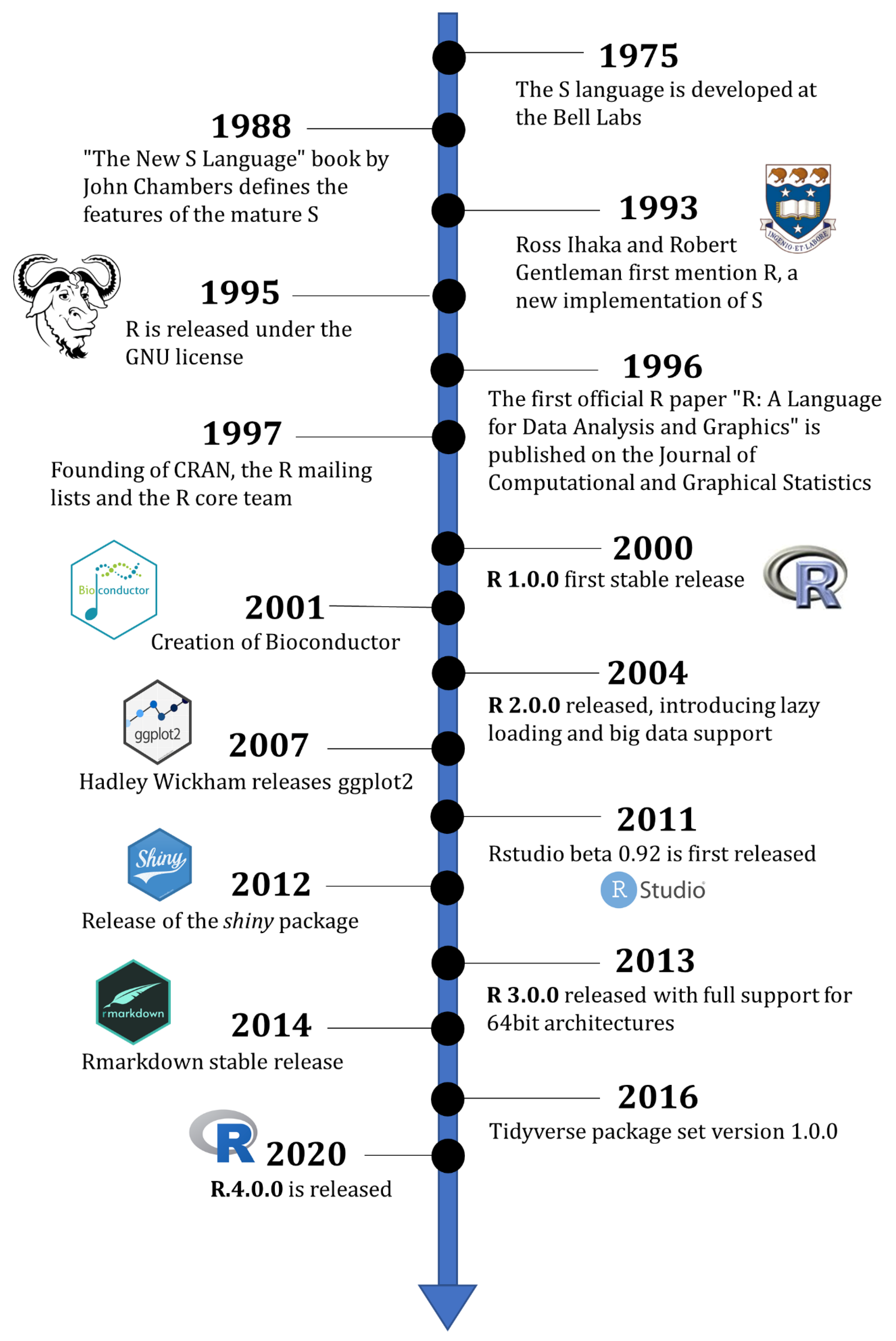
Figure 1.1: Short history of R from Giorgi, Ceraolo, and Mercatelli (2022).
A more detailed history of R development and first objectifs.
1.1.2 Why R?
It is hard to answer this question in one sentence. But several points can be raised :
- The non-cost of this software compared to heavy ones from other platforms.
- The high number of packages developed and freely available allows more and more analysis in many fields of applications.
- As depicted in Tippmann (2015) the idea of knowing “what you are doing to your data” and not having a black box treatment of your data.
- Mastering the whole chaine opératoire from the cleaning of your raw data to the publishing of reports or graphics.
- Allows others to see your code and treatment “the reproducibility of the experiment”.
- One of the most used programming languages, in the top 20 of the TIOBE Index for many years.
![Number of publications quoting R [@tippmann_programming_2015].](images/R_publication.png)
Figure 1.2: Number of publications quoting R (Tippmann 2015).
1.2 Resources
The R community is well developed online and you can found many resources on several websites.
For the basics resources you have:
- https://cran.r-project.org/: R original deposit of the CRAN.
- https://rstudio.com/products/rstudio/: Rstudio is the most commonly used IDE for R.
- https://Github.com: GitHub, a website with developers’ codes and packages freely accessible. Also some topics about issues and bugs in R.
To solve coding problems and bugs:
- https://r-grrr.slack.com/ Slack of R users (question/answers, actuality…).
- https://www.r-bloggers.com/ R-bloggers.
- https://stackoverflow.com/questions/tagged/r/ Stackoverflow (very useful).
1.3 Installing R and dependencies
1.3.1 R and Rstudio
First, you will need to install R on https://cran.r-project.org/. Choose the fitted version for your computer system.
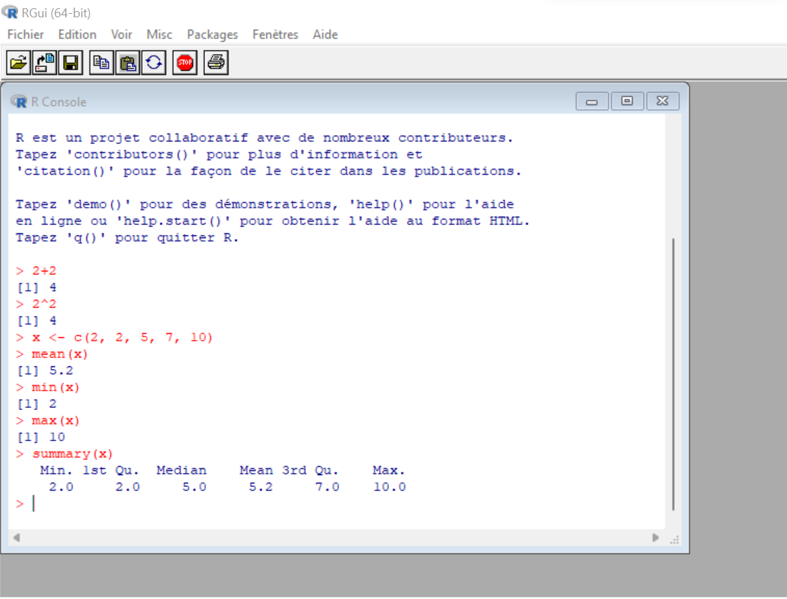
Figure 1.3: R software view.
Then you will need an Integrated Development Environment (IDE) which allows you to have a more comprehensive overview and easier access to packages and other online features from R. The most commonly used IDE for R is Rstudio. You can download it via https://posit.co/download/rstudio-desktop/, and select the free version for your exploitation system.
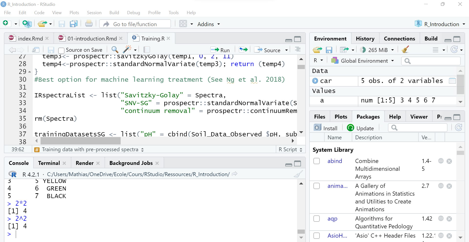
Figure 1.4: RStudio IDE view.
1.3.2 R Packages
If basic R already handles many data, the true power of this language is to have more than 10 000 additional updated packages freely available online. Most of them can be directly downloaded on the CRAN website while others will be accessible only via their GitHub deposit.
To download the package you have several different solutions:
- The easiest way is using the Package windows of Rstudio and directly downloading it from the CRAN deposit.
- You can also use the following code to download it
install.packages(""). - If the package is not available on the CRAN deposit you can directly download it from the GitHub site. You will need first to download the “remote” package to access online content. Then you can type the URL of the link to your package.
install.packages("remotes") #install "remotes" package.
devtools::install_github("philipp-baumann/simplerspec", force = FALSE) # The "force" parameter (TRUE or FALSE) depending if you want to overwrite your previous download of the package- Last but not least, you can manually download the
.zipor.tar.gzof the package online and unpacked it via the package windows of Rstudio or directly to your R folder (1.5)
Once you download the package you have to load it to your environment. You can do it with the line library() , you will have to do it every time you start a new session in R.
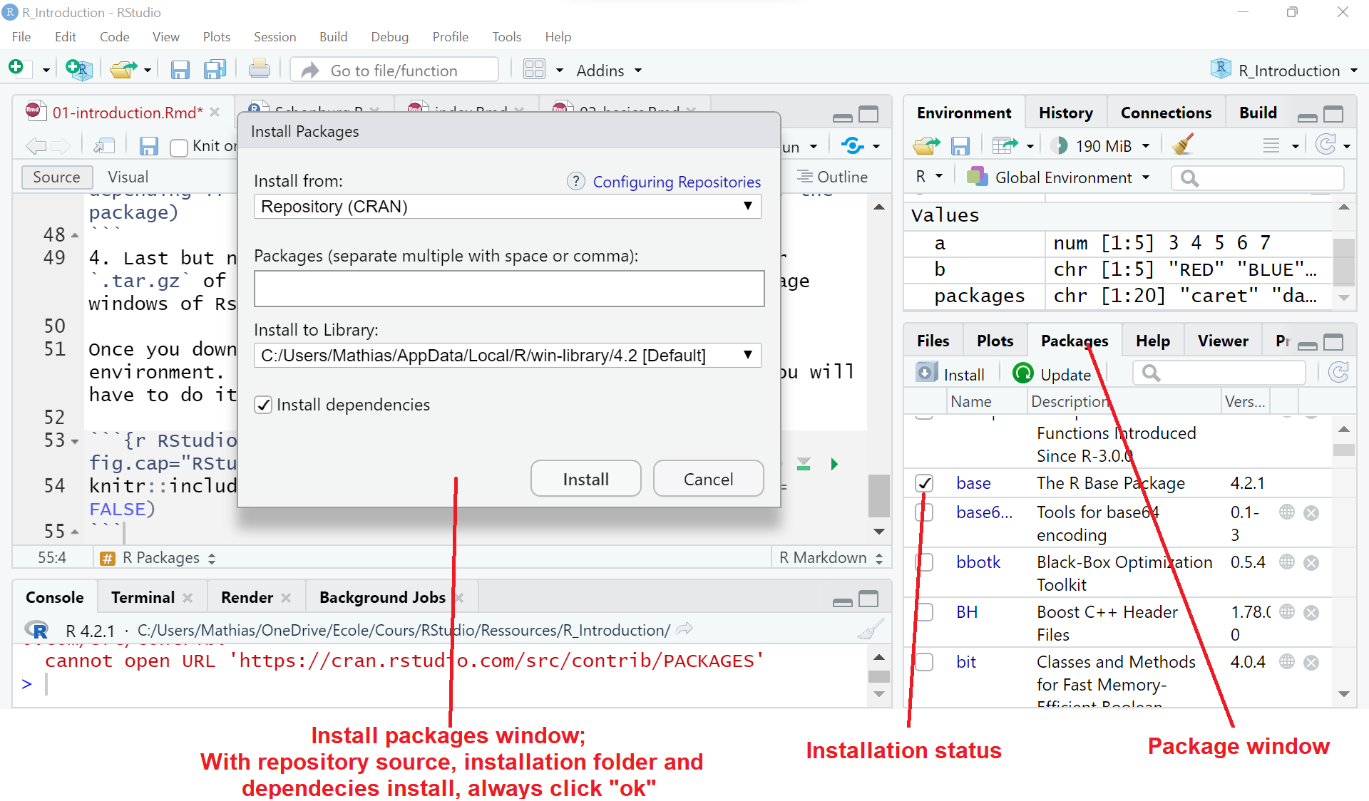
Figure 1.5: RStudio Package window view.
1.4 First overview of R
1.4.1 Basic commands
You can open a new R window to start typing some code lines.
R is based on statistical treatment so numbers and operations are one of the most important components of this language. You can type basic operations to get familiar with the syntax:
Special operators can also be used.
For letters and other characters you can use the print()command. It does work for special operators but not if several are used at the same time.
> print("Hello World")
[1] "Hello world"
> print(pi)
[1] 1.414214
> print("The zero occurs at", 2 * pi, "radians.")
Error in print.default("The zero occurs at", 2 * pi, "radians."):
invalid 'quote' argument
To be able to use both numeric or special operators and characters, use the cat() command. You need to end it with the "\n" code.
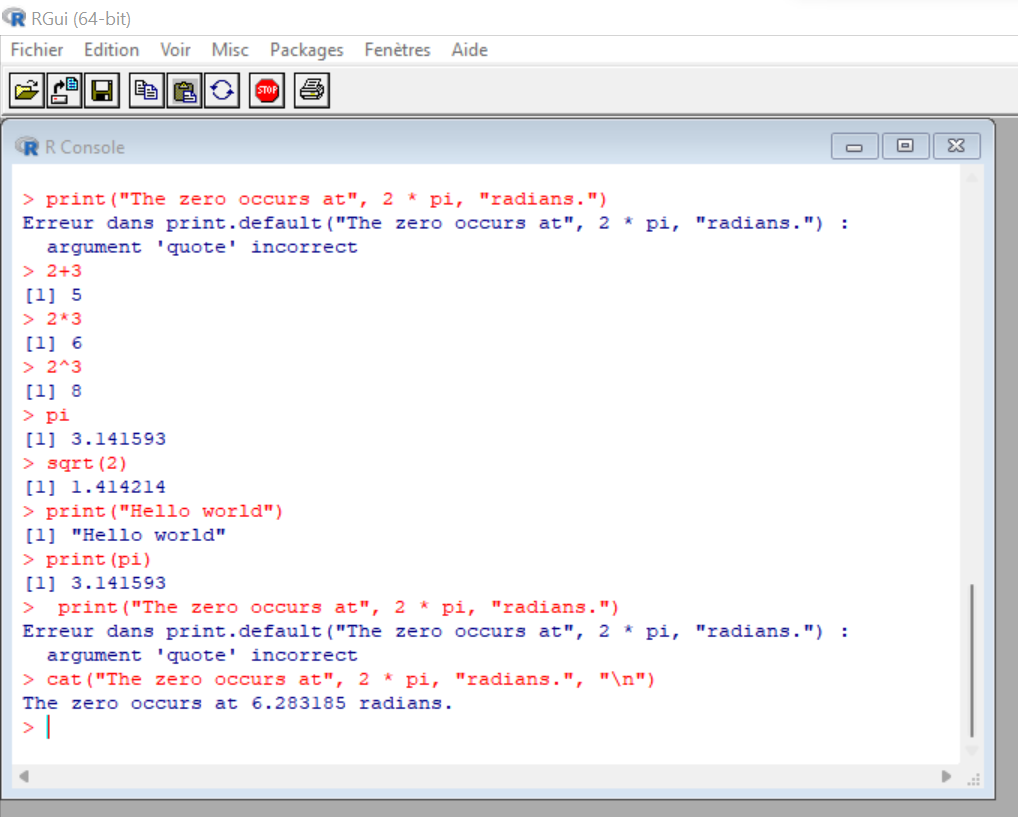
Figure 1.6: R basic commands.
An important topic is the help() command (in Rstudio ? can also work). This function will give access to the description of the command you are typing inside the strings. With an internet connection on Rstudio the ?? line will give you information on your command even if it is coming from a non-downloaded package.
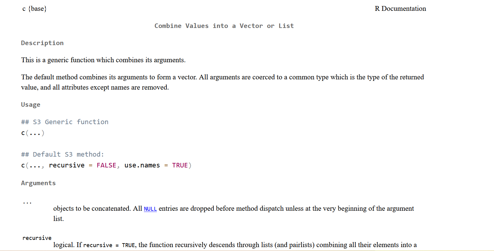
Figure 1.7: R help window after typing the help(c) command.
1.4.2 Setting variables
Analyzing data is important but if we can not store them we won’t be able to go very far. You can store any variable with the <- or = code. The most important variables are numbers and character strings.
Numerical values
On the upper code line, it is a number variable storage (Numeric values).
> a <- "The zero occurs at"
> b = "radians."
> cat(a, 2 * x, b, "\n")
The zero occurs at 6.283185 radians.
Character values
On the upper code line, it is two character string variables storage (Character values) combined with a number variable.
We can also give a vector several numbers (Vector of numbers) or several characters (Vector of character strings) with the code line c().
> a <- c("Red", "Blue", "Green", "Black", "White")
> b <-  c(5, 6, 6, 8, 11)
> print(a)
[1] "Red"   "Blue"  "Green" "Black" "White"
> b
[1]  5  6  6  8 11
Useful commands
You have to distinguish the class of data from its mode. The class can be seen as the structure of the data while the mode is just the “type” of data. In simple vectors there is no difference but on more complex objects you will have a specific class for the all structure (matrices, arrays…) while the data stored inside will be related to one or several mode (numeric, character, logical…) To know the class of your variable you can use the class()command and to know the mode (type of info stored) the mode(). The str() function will give you more information about the data and its class.
> str(a)
[1] chr [1:5] "Red" "Blue" "Green" "Black" "White"
> class(b)
[1] "numeric"
> mode(print)
[1] "function"
Two other important commands are ls() which gives you your number of saved variable and rm() which remove one variable. ls.str() is a transformed way to see the content of each variable and not only there name. You can remove all your variable by making rm(list = ls()). The c(1:10) used here gives a vector list of ten numbers from 1 to 10. The : function create a sequence of numbers.
> y <- 3
> y <- "Red"
> z <- c(1:10)
> ls()
[1] "x" "y" "z"
> ls.str()
x :  num 3
y :  chr "RED"
z :  int [1:10] 1 2 3 4 5 6 7 8 9 10
> rm(list = ls())
> ls()
character(0)
To generate a more “complex” sequence you can use the seq(x, y, n) function where x is the starting number, y is the ending number and n is the interval. If you want to create a sequence with a specific number of intervals you can use the length.out = argument before n.
> seq(2, 50, 4)
 [1]  2  6 10 14 18 22 26 30 34 38 42 46 50
> seq(2, 50, length.out = 4)
[1]  2 18 34 50
Matrices and Arrays
You can combine vectors together in order to create matrices the first time. There are different ways of combining them. When can combine the different vector numbers with c() and then give a specific dimension x,y to the combined vector with dim(x,y) command. Or we can directly combine the two vectors as different columns from one matrix with cbind(col1, col2) or if you prefer combine via the rows with rbind(row1, row2). Another possible way is with matrix(data, nrow = n, ncol = n).
> b <- c(5, 6, 6, 8, 11)
> d <- c(12, 3, 4, 5, 6)
> matrix <- c(b,d)
> matrix
[1]  5  6  6  8 11 12  3  4  5  6
> dim(matrix) <- c(2,5) # first the rows number then the columns number
> print (matrix)
     [,1] [,2] [,3] [,4] [,5]
[1,]    5    6   11    3    5
[2,]    6    8   12    4    6

> matrix <- cbind(b, d)
> print(matrix)
      b  d
[1,]  5 12
[2,]  6  3
[3,]  6  4
[4,]  8  5
[5,] 11  6
> dim(matrix)
[1] 5 2

> matrix <- rbind(b, d)
> print(matrix)
     [,1] [,2] [,3] [,4] [,5]
[1,]    5    6   11    3    5
[2,]    6    8   12    4    6
> dim(matrix)
[1] 2 5
> class(matrix)
[1] "matrix" "array"
The type array is a multidimensional n vectors. We will prefer data frame format or list format for combining different types of data. However, if you want more precision on array data you can look into Long and Teetor (2019) pp.131 - 132 or Team, Venables, and Smith (2022).
Factor values
Another type of important data is the factor class. They are defined as a vector of enumerated values. There is two type of factor the Grouping and the Categorical variables which are commonly used for ANOVA testing. The specificity of the factor is that they contain several levels (one for each type of factor). You can access the levels with levels()to see their names or nlevels()to see the number of levels.
Transformation
You can force R to convert data from a previous class to another with the as.x() code where x is replaced by the format (data frame, numeric, character….). In our case here you can ask as.factor().
> x <- factor(c("TRUE","FALSE","TRUE","TRUE","FALSE","NO DATA","TRUE", "FALSE"))
> class(x)
[1] "factor"
> levels(x)
[1] "FALSE"   "NO DATA" "TRUE"
> a <- c("Red", "Blue", "Green", "Black", "White")
> y <- as.factor(a)
> nlevels(y)
[1] 5               #one for each type of character
You can also order factors by adding the ordered = TRUE code inside the factor() function. This can be useful when sorting the data you are dealing.
> x <- factor(c("TRUE","FALSE","TRUE","TRUE","FALSE","NO DATA","TRUE", "FALSE"))
> sorted <- factor(x, ordered = TRUE, levels = c("NO DATA", "FALSE",  "TRUE"))
> sorted
[1] TRUE    FALSE   TRUE    TRUE    FALSE   NO DATA TRUE    FALSE
Levels: NO DATA < FALSE < TRUE
Lists and data frames
Two very common data types we will see here are List and Data Frame. A list can be seen as a collection of objects. They can be from different modes and sizes without any restrictions except for having different names. The data frame (more broadly used in Data Science) can be seen as a specific type of list with two conditions :
- All elements of a data frame are vectors.
- All elements of a data frame have an equal length.
For a list, you can type the list() code. The detail code is list(name_1 = object_1, …, name_m = object_m). The data frame looks similar to the list() function. You can write it down with the data.frame() code line. If you try to create a data frame with an unequal number between vectors it will notice it.
> Lst <- list(name="Fred", wife="Mary", no.children=3,
child.ages=c(4,7,9))
> str(Lst)
List of 4
 $ name       : chr "Fred"
 $ wife       : chr "Mary"
 $ no.children: num 3
 $ child.ages : num [1:3] 4 7 9
>
> df <- data.frame(id=1:3, name=c("Moe", "Larry", "Curly"), age=c(1:3))
>str(df)
'data.frame':   3 obs. of  3 variables:
 $ id  : int  1 2 3
 $ name: chr  "Moe" "Larry" "Curly"
 $ age : int  1 2 3
>
> df <- data.frame(id=1:3, name=c("Moe", "Larry", "Curly"), age=c(1,2))
Error in data.frame(id = 1:3, name = c("Moe", "Larry", "Curly"), age = c(1,  :
    arguments imply differing number of rows: 3, 2
This example is from the Team, Venables, and Smith (2022) book.
Logical and Integer values
You have also logical values that can be “TRUE”, “FALSE” or “NULL”. You create them with a vector command and then T, F or N without strings c(T,F,F,N). There are useful values for logical comparison between two variables (See vector operator).
Integer values can also be created by adding the as.integer code on a numerical vector. By default numerical values are non integers in R.
> x <- c(T,F,T,F,T,N)
> class(x)
[1] "logical"
> y <- 2000 > 2022
> class(y)
[1] "logical"

> b <- c(5, 6, 6, 8, 11)
> b_int <- as.integer(b)   #Integer will truncated toward zero non integral number and imaginary part of complex numbers will be discarded.
> class(b_int)
[1] "integer"| Object | Example | Mode |
|---|---|---|
| Number | 3.1415 | Numeric |
| Vector of numbers | c(2.7.182, 3.1415) | Numeric |
| Character string | “Moe” | Character |
| Vector of character strings | c(“Moe”, “Larry”, “Curly”) | Character |
| Factor | factor(c(“NY”, “CA”, “IL”)) | Numeric |
| List | list(“Moe”, “Larry”, “Curly”) | List |
| Data frame | data.frame(x=1:3, y=c(“Moe”, “Larry”, “Curly”)) | List |
| Function | print() | Function |
| Logical values | c(T,F,F,F,T,T) | Logical |
1.5 RStudio Environment
1.5.1 Project
When you are opening a new project create a new project in the tab File and then create an R script in new file in the tab File. Choose carefully your project folder because it will be more complicated to move it later on.
Treeing
The organization of the folder is also really important you can read this blog (https://www.inwt-statistics.com/read-blog/a-meaningful-file-structure-for-r-projects.html) about the organisation of a project folder and look the snapshot below 1.8.
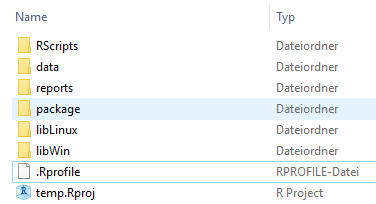
Figure 1.8: R project folder structure.
You have several ways of controlling your folder location with getwd() and setting a new one with setwd(). The formula ./ will automatically call the project folder. Note that when your a calling any path into R you will need / and not \ as commonly used in windows or other programming languages (Cf. Latex)
1.5.2 Saving the data
For saving your working space you have two ways:
- Either export one by one your file to specific formats (.csv, .jpg, .shp….) as we will see later.
- Saving via a .RData the file is more easily readable on R. You can save only one or multiple elements
save(list = c("x","y"), file = "output.RData")or all environment of your projectsave.image(file = "output.RData").
1.6 Exercices
- Calculate the following equation with R and copy the code lines:
\[ x = (2*4-4)^2 + \sqrt(9) \]
- Solve the following equation rounded at 3 digits (if necessary) by using the quadratic formula: \[ -5x^2 - 6x + 11 = 2 \] For reminder the quadratic formula : \[ ax^2 + bx + c = 0 \]
\[ x = \frac{-b \pm \sqrt{b^2 - 4ac}}{2a} \]
Create 5 vectors (minimum length 3) from different classes. Name them after their class name and export them as a list in a .RData file named Exercise_R_01.
Give the objects class, variable mode and number, and observation number of the data
rock,treesandiris. These data are included in R basic package.
See solution
## [1] 19## [1] -2.069694## [1] 0.8696938## 'data.frame': 48 obs. of 4 variables:
## $ area : int 4990 7002 7558 7352 7943 7979 9333 8209 8393 6425 ...
## $ peri : num 2792 3893 3931 3869 3949 ...
## $ shape: num 0.0903 0.1486 0.1833 0.1171 0.1224 ...
## $ perm : num 6.3 6.3 6.3 6.3 17.1 17.1 17.1 17.1 119 119 ...## 'data.frame': 31 obs. of 3 variables:
## $ Girth : num 8.3 8.6 8.8 10.5 10.7 10.8 11 11 11.1 11.2 ...
## $ Height: num 70 65 63 72 81 83 66 75 80 75 ...
## $ Volume: num 10.3 10.3 10.2 16.4 18.8 19.7 15.6 18.2 22.6 19.9 ...## 'data.frame': 150 obs. of 5 variables:
## $ Sepal.Length: num 5.1 4.9 4.7 4.6 5 5.4 4.6 5 4.4 4.9 ...
## $ Sepal.Width : num 3.5 3 3.2 3.1 3.6 3.9 3.4 3.4 2.9 3.1 ...
## $ Petal.Length: num 1.4 1.4 1.3 1.5 1.4 1.7 1.4 1.5 1.4 1.5 ...
## $ Petal.Width : num 0.2 0.2 0.2 0.2 0.2 0.4 0.3 0.2 0.2 0.1 ...
## $ Species : Factor w/ 3 levels "setosa","versicolor",..: 1 1 1 1 1 1 1 1 1 1 ...1.7 Additionnal Ressources
Here you will find videos or links for additional material.
Philosophy of R and free software
- https://www.youtube.com/watch?v=jk9S3RTAl38 : John Chambers interview on the R and S language philosophy and origin.
- https://www.youtube.com/watch?v=Ag1AKIl_2GM : Richard Stallman TEDx on the free softwares.
- John M. Chambers, “S, R and Data Science”, The R Journal, 12:1, 2020, pp. 462-476.
- Chamber, John M., Programming with Data: A Guide to the S Language, Springer, 1998.
History of R language
- Becker, Richard A., A Brief History of S, Murray Hill, New Jersey: AT&T Bell Laboratories, 2015.
- https://www.youtube.com/watch?v=Uey45MSg8Y4 : Peter Dalgaard conference on history of R in CeleBration 2020 in Copenhagen, 2020.
- https://www.youtube.com/watch?v=qWG_MLrxKps&t :John Chambers talk about S, R and Data Science short history, 2021.
Why R?
- https://www.youtube.com/watch?v=4lcwTGA7MZw&t : Short presentation on R pros and cons compared to python.
- Giorgi, Frederico, Ceraolo Carmine, Mercatelli Daniele, “The R Language: An Engine for Bioinformatics and Data Science”, Life, 12, 648, 2022.
Formation online
- Basic an quick online course (4 - 6 hours) : https://courses.cognitiveclass.ai/courses/course-v1:CognitiveClass+RP0101EN+v1/course/
- More developed course about many uses of R (8 - 10 hours) : https://learning.edx.org/course/course-v1:HarvardX+PH125.1x+1T2022/home