2 Conditioned Latin hypercube sampling
2.1 Introduction
2.1.1 Purpose
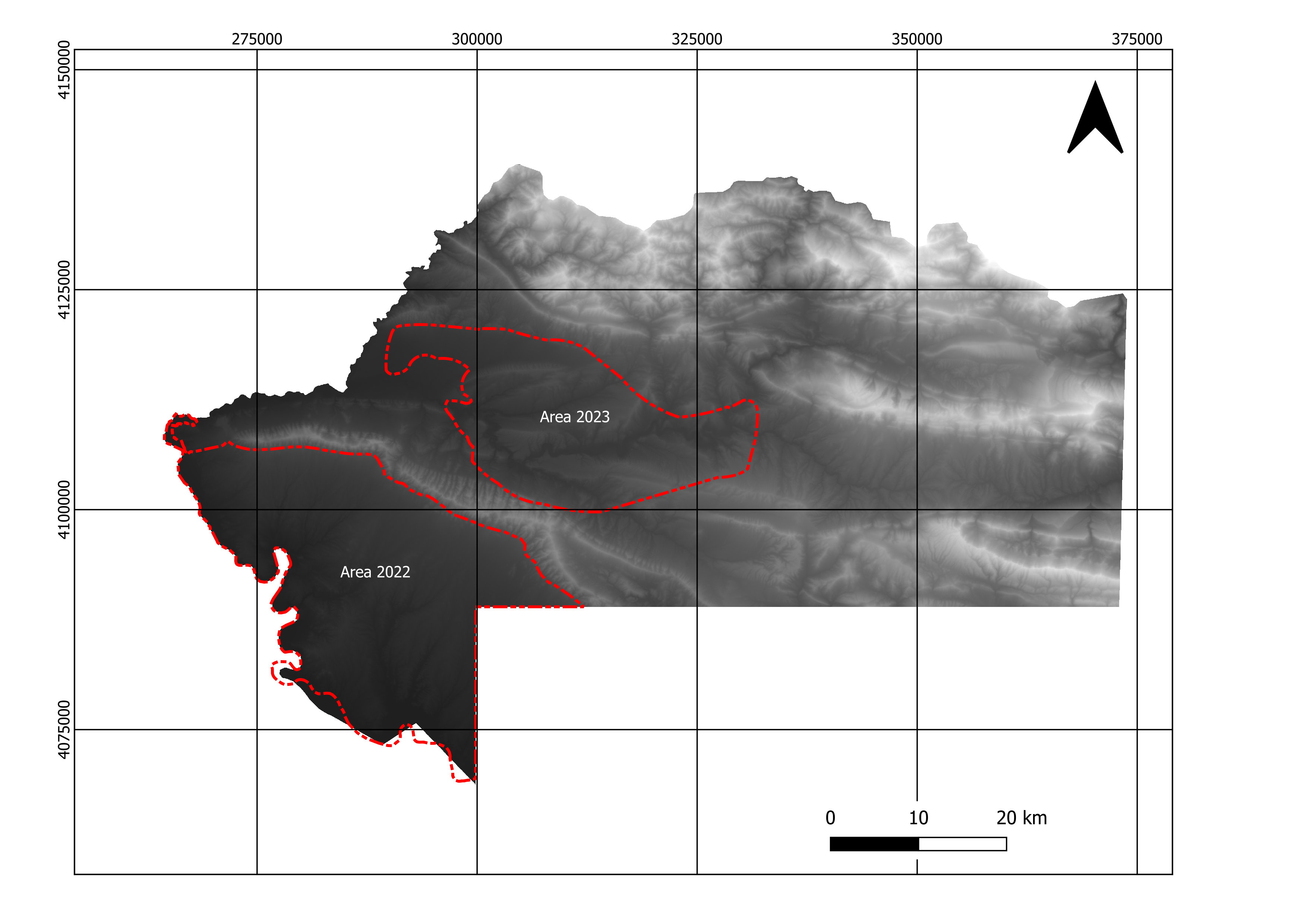
This document presents the results of the sampling design for the 2022 and 2023 summer field campaigns of the B07 subproject in CRC1070. We used a specific sampling technique called conditioned Latin hypercube sampling (cLHS). This sampling strategy based on combinations of different strata/layers gave a diversity of samplings according to the heterogeneity of the layers. We tried different numbers of sampling locations (100, 150, 200, 250, 300, 350 and 400) to finally agree on a set of 100 samplings (We majored the number of samples by 10% - to reach 110 locations - to avoid any issue on the file in case of non-accessible area). The study area covers over 830 km\(^2\) in 2022 and 490 km\(^2\) in 2023. The size of area C explored in 2023 is equal to 1450 km\(^2\). Still, due to inaccessible places in high mountains or conflict zones between PKK (Kurdistan Workers’ Party) and the Turkish army (Ertan 2022), we reduce the explored area.
2.1.2 Procedure
We first produced several maps composed of different factors before using them as layers for the conditioned Latin hypercube sampling. We used different software such as GIS 3.24.1 version and SAGA GIS 7.8.2, GoogleEarthEngine (GEE) and R 4.4 with Rstudio. The procedure is partially based on the Sampling package from Dick Brus and its reference book (Brus 2022).
2.1.3 Input data
All the data listed below are available freely online excepted for the digitized maps (geomorphology).
| Name/ID | Original resolution (m) | Type/Unit | Source |
|---|---|---|---|
| DEM/TE.5 | 25 | Meters | ESA and Airbus (2022) |
| RUSLE map/OT.11 | 25 | Mg/ha\(^{-1}\) year\(^{-1}\) | Mathias Bellat |
| Slope/TE.16 | 25 | Radians | ESA and Airbus (2022) |
| TWI/TE.22 | 25 | - | ESA and Airbus (2022) |
| Soil estimation/OT.12 | 10 | - | Nafiseh Kakhani / USGS (2018) |
| Geomorphology/OT.3 | 1 : 250 000 | - | Forti et al. (2021) |
| Landsat 8 Green/LA.3 | 30 | 0.53 - 0.59 µm | USGS (2018) |
| Landsat 8 Red/LA.4 | 30 | 0.64 - 0.67 µm | USGS (2018) |
| Landsat 8 NIR/LA.5 | 30 | 0.85 - 0.88 µm | USGS (2018) |
| Landsat 8 SWIR1/LA.6 | 30 | 1.57 - 1.65 µm | USGS (2018) |
| Landsat 8 SWIR2/LA.7 | 30 | 2.11 - 2.29 µm | USGS (2018) |
2.2 Data treatement
2.2.1 Soil prediction map
The Landsat 8 images were collected via a Google Earth Engine script on a period covering 2020, the median of the composite image from Tier 1 TOA collection was used. To produce the soil estimation map we based our prediction on a Google Earth Engine written script. The javascript codes for scraping these images and computing the soil estimation indexes are available in the supplementary file inside the “2 - CLHS/code” folder. We computed four soil indexes:
\[ Landsat~8~Clay~index = \frac{SWIR1}{SWIR2} \] Hengl (2007), USDA/GO (former GTAC)
\[ Landsat~8~Ferrous~minerals~ratio = \frac{SWIR1}{NIR} \]
Al-Mousawi, Fouad, and Sissakian (2007), Henrich et al. (2012) (Ferric Oxides), USDA/GO (former GTAC)
\[ Landsat~8~Carbonate~index = \frac{Red- Green}{Red +Green} \]
Pouget et al. (1991) (Color, Hematite/ goethite), USDA/GO (former GTAC)
\[ Landsat~8~Rocks~outcrop~index = \frac{SWIR1-Green}{SWIR1+Green} \]
USDA/GO (former GTAC)
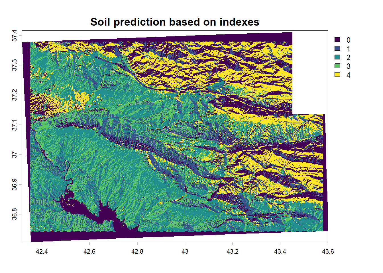
(#fig:erosion map recall)Soil prediction based on indexes (WGS84, UTM38N).
2.2.2 Soil erosion based on RUSLE model
The RUSLE map was previously computed in Chapter 1.
2.2.3 DEM, slope and topographic wetness index
The DEM is on a 30 x 30 m scale based on the ESA data (ESA and Airbus 2022). The slope under SAGA GIS 7.8.2 with the function Slope, Aspect, Curvature with the method by Zevenbergen, L.W., Thorne, C.R. (1987). For the topographic wetness index the Topographic Wetness Index (One step) command was used with Multiflow direction parameters
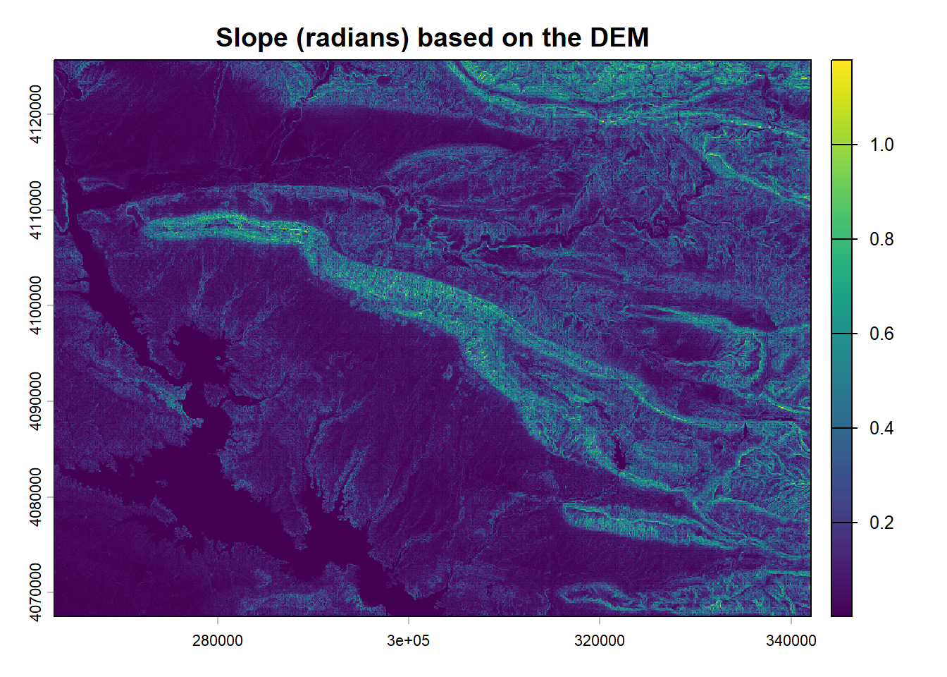
(#fig:slope map)Slope (radians) based on the DEM (WGS84, UTM38N).
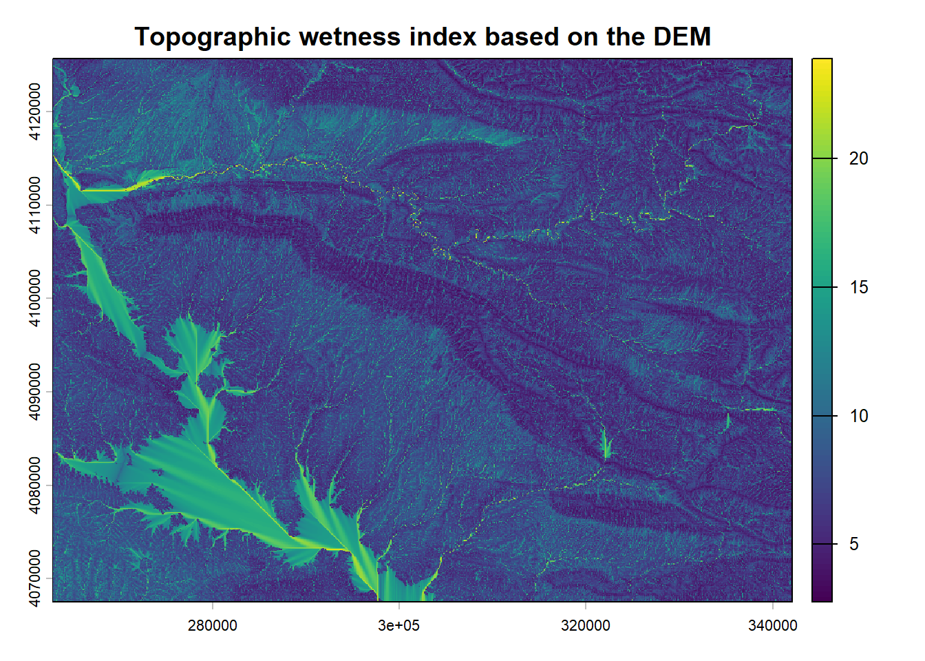
(#fig:TWI map)Topographic wetness index based on the DEM (WGS84, UTM38N).
2.2.4 Geomorphological map
The geomorphological map is computed based on (Forti et al. 2021). We created 17 different layers for each of the geomorphons present.
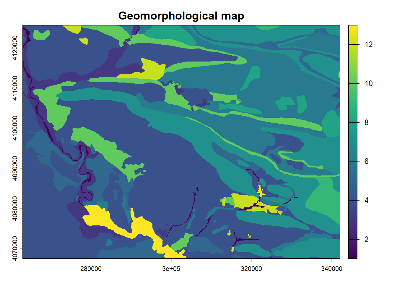
(#fig:geomorpho map)Geomorphological map (WGS84, UTM38N).
2.3 Conditioned Latin hypercube sampling script
2.3.1 Preparation of the R environement
# 0 Environment setup ##########################################################

# 0.1 Prepare environment ======================================================
# Folder check
getwd()

# Select folder
setwd(getwd())

# Clean up workspace
rm(list = ls(all.names = TRUE))

# 0.2 Install packages =========================================================

# Load packages
library(pacman) #Easier way of loading packages
pacman::p_load(sf, mapview,raster, clhs) # Specify required packages and download it if needed

# 0.3 Show session infos =======================================================
sessionInfo()
R version 4.5.1 (2025-06-13 ucrt)
Platform: x86_64-w64-mingw32/x64
Running under: Windows 11 x64 (build 26200)
Matrix products: default
LAPACK version 3.12.1
locale:
[1] LC_COLLATE=French_France.utf8 LC_CTYPE=French_France.utf8 LC_MONETARY=French_France.utf8 LC_NUMERIC=C
[5] LC_TIME=French_France.utf8
time zone: Europe/Paris
tzcode source: internal
attached base packages:
[1] grid parallel stats graphics grDevices utils datasets methods base
other attached packages:
[1] clhs_0.9.2 raster_3.6-32 sp_2.2-0 mapview_2.11.4 sf_1.0-24
loaded via a namespace (and not attached):
[1] splines_4.5.1 tibble_3.3.1 cellranger_1.1.0 hardhat_1.4.2 pROC_1.19.0.1 rpart_4.1.24
[7] lifecycle_1.0.5 tcltk_4.5.1 SpaDES.tools_2.1.1 globals_0.18.0 lattice_0.22-7 MASS_7.3-65
[13] crosstalk_1.2.2 backports_1.5.0 magrittr_2.0.4 rmarkdown_2.30 yaml_2.3.12 otel_0.2.0
[19] lobstr_1.1.3 reproducible_3.0.0 gld_2.6.8 bayesm_3.1-7 DBI_1.2.3 lubridate_1.9.4
[25] expm_1.0-0 purrr_1.2.1 nnet_7.3-20 tensorA_0.36.2.1 ipred_0.9-15 gdtools_0.4.4
[31] satellite_1.0.6 lava_1.8.2 listenv_0.10.0 terra_1.8-93 units_1.0-0 parallelly_1.46.1
[37] svglite_2.2.2 codetools_0.2-20 xml2_1.5.2 Require_1.0.1 tidyselect_1.2.1 quickPlot_1.0.4
[43] farver_2.1.2 stats4_4.5.1 base64enc_0.1-3 e1071_1.7-17 survival_3.8-6 iterators_1.0.14
[49] systemfonts_1.3.1 foreach_1.5.2 tools_4.5.1 Rcpp_1.1.1 glue_1.8.0 Rttf2pt1_1.3.14
[55] prodlim_2025.04.28 gridExtra_2.3 qs2_0.1.7 xfun_0.56 dplyr_1.1.4 withr_3.0.2
[61] fastmap_1.2.0 boot_1.3-32 digest_0.6.39 timechange_0.3.0 R6_2.6.1 textshaping_1.0.4
[67] dichromat_2.0-0.1 generics_0.1.4 fontLiberation_0.1.0 data.table_1.18.0 recipes_1.3.1 robustbase_0.99-6
[73] class_7.3-23 httr_1.4.7 htmlwidgets_1.6.4 whisker_0.4.1 ModelMetrics_1.2.2.2 pkgconfig_2.0.3
[79] gtable_0.3.6 Exact_3.3 timeDate_4051.111 rsconnect_1.7.0 S7_0.2.1 sys_3.4.3
[85] htmltools_0.5.9 fontBitstreamVera_0.1.1 bookdown_0.46 SpaDES.core_3.0.4 scales_1.4.0 lmom_3.2
[91] png_0.1-8 gower_1.0.2 knitr_1.51 rstudioapi_0.18.0 tzdb_0.5.0 reshape2_1.4.5
[97] checkmate_2.3.3 nlme_3.1-168 proxy_0.4-29 stringr_1.6.0 rootSolve_1.8.2.4 KernSmooth_2.23-26
[103] extrafont_0.20 pillar_1.11.1 vctrs_0.7.0 stringfish_0.18.0 cluster_2.1.8.1 extrafontdb_1.1
[109] evaluate_1.0.5 readr_2.1.6 mvtnorm_1.3-3 cli_3.6.5 compiler_4.5.1 rlang_1.1.7
[115] future.apply_1.20.1 classInt_0.4-11 plyr_1.8.9 forcats_1.0.1 fs_1.6.6 stringi_1.8.7
[121] fpCompare_0.2.4 leaflet_2.2.3 fontquiver_0.2.1 pacman_0.5.1 Matrix_1.7-4 hms_1.1.4
[127] leafem_0.2.5 future_1.69.0 ggplot2_4.0.1 haven_2.5.5 igraph_2.2.1 RcppParallel_5.1.11-1
[133] DEoptimR_1.1-4 readxl_1.4.5 2.3.2 Preparation of the data
# 1 Import and prepare the data  -----------------------------------------------
# 1.1 Select the the files #####################################################
Area <- st_read("./data/Sampling_area_2022.gpkg", layer = "Sampling_area_2022")  # Change the area for 2022 and 2023 campaigns
DEM <- rast("./data/DEM.tif")
Geomorpho <- rast("./data/Geomorphology.tif")
Soil_erosion <- rast("./data/RUSLE_map.tif")
Soil_prediction <- rast("./data/Soil_prediction.tif")
Slope <- rast("./data/Slope.tif")
Wetness <- rast("./data/TWI.tif")

# 1.2 Clean and prepare the DEM ################################################

# Crop the DEM to the study area
DEM <- crop(DEM, Area, inverse=FALSE, updatevalue=NA, updateNA=TRUE)

# Mask the DEM to the study area
DEM <- mask(DEM, Area, inverse=FALSE, updatevalue=NA, updateNA=TRUE)

# 1.3 Clean and prepare the covariates #########################################

# Create a list of the different variables
list <- list(Geomorpho, Soil_erosion, Soil_prediction, Slope, Wetness)
names(list) <- c("Geomorpho","Soil_erosion","Soil_prediction","Slope", "Wetness")

# Set the CRS WGS84 UTM38N to all raster
ZoneUTM <- c("+init=epsg:32638")
for (i in names(list)) {
  r <- list[[i]]
  list[[i]] <- projectrast(r, crs = ZoneUTM)
}

# Resample according to the DEM
# With NGB only for the categorical raster
list[[1]]  <- resample(list[[1]], DEM, "ngb")
list[[3]]  <- resample(list[[3]], DEM, "ngb")

# With bilinear only for the numerical raster
list[[2]]  <- resample(list[[2]], DEM, "bilinear")
list[[4]]  <- resample(list[[4]], DEM, "bilinear")
list[[5]]  <- resample(list[[5]], DEM, "bilinear")

# 1.4 Stack all the predictors #################################################
stack <- stack(DEM, list$Geomorpho, list$Soil_erosion,list$Soil_prediction,
              list$Slope, list$Wetness)  # stack all the data in a stacked raster

plot(stack$DEM)
# 1.5 Save and export the predictors ###########################################
writerast(stack ,filename = "./export/predictors.tif", format="GTiff",overwrite=T)

rm(list = ls())
2.3.3 Calculation of the conditioned Latin hypercube sampling
# 2 Create the Conditioned Latin Hypercube Sampling  ---------------------------
# 2.1 Import and prepare the files #############################################
predictors <- raster::stack("./export/predictors.tif")
names(predictor@layers) <- c("DEM","Geomorpho","Soil_erosion","Soil_prediction","Slope", "Wetness" )

# Convert the file into Data Frame
PredForMap  <- as(predictors, 'SpatialPixelsDataFrame')
PredForMap <- data.frame(PredForMap)
stack_frame <- PredForMap[complete.cases(PredForMap),] # Remove NA values

names(stack_frame) <- c("DEM","Geomorpho","Soil_erosion","Soil_prediction","Slope", "Wetness", "x", "y")
stack_frame$Geomorpho <- round(stack_frame$Geomorpho, digits=0) # If ever the categorical classification did not work
stack_frame$Soil_prediction <- round(stack_frame$Soil_prediction, digits=0) # If ever the categorical classification did not work
stack_frame <- na.omit(stack_frame)

save.image("./export/Pre-process.RData") # Save the image

# 2.2 Conditioned Latin Hypercube sampling parameters ##########################

# Select the predictors for the Conditioned Latin Hypercube
preds <- c("DEM","Geomorpho","Soil_erosion","Soil_prediction","Slope","Wetness")

# Set the size of the sampling
c = 110

# Set a seed
set.seed(1070)

# Run the sampling
res <- clhs(stack_frame[, preds], size = c,  tdecrease = 0.95, iter = 50000, progress = FALSE, simple = FALSE)

# 2.3 Export the results #######################################################

# Fit the results with the line in the table
CLHS_sampled_res <- stack_frame[res$index_samples, ]
# Convert to spatial data frame point
CLHS_sampled_df <- SpatialPoints(coords =  CLHS_sampled_res[, c("x", "y")], proj4string=CRS("+init=epsg:32638"))

# Export the results in a CSV format
write.table(CLHI_sampled_df, "./export/CLHS_2022.csv", col.names = TRUE, sep = ";", row.names = FALSE,
          fileEncoding = "UTF-8") #Replace 2022 with 2023 for the 2023 summer sampling campaign
2.4 Sampling locations
Some sampling locations were located in inaccessible areas so not all the spots have been sampled. Only 101 in 2022 and 21 in 2023. Despite this lack of few samples sites, the distribution of the cLHS variables was similar to better than a classical random sampling method.
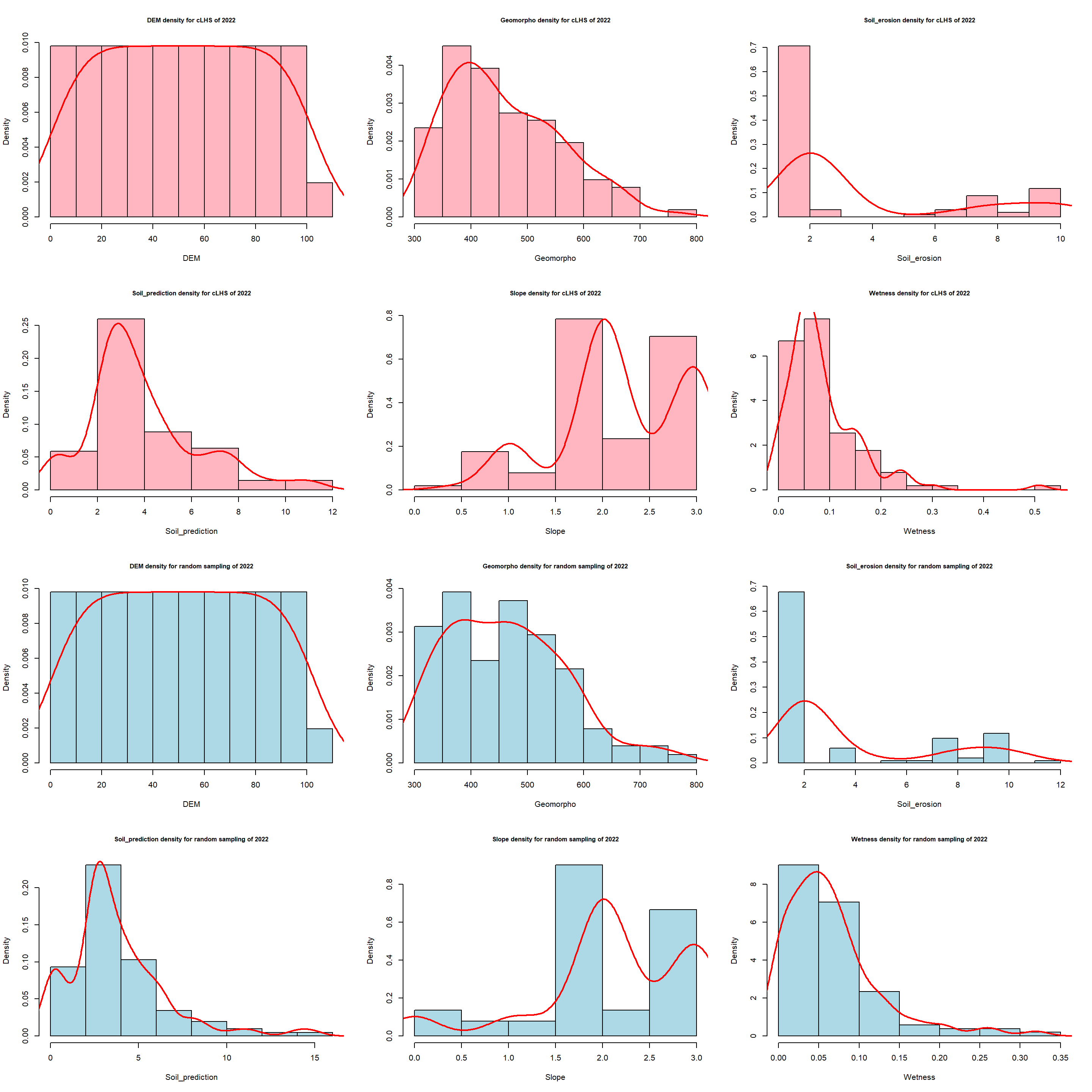
(#fig:density samples 2022)2022 Campaign samples distribution.
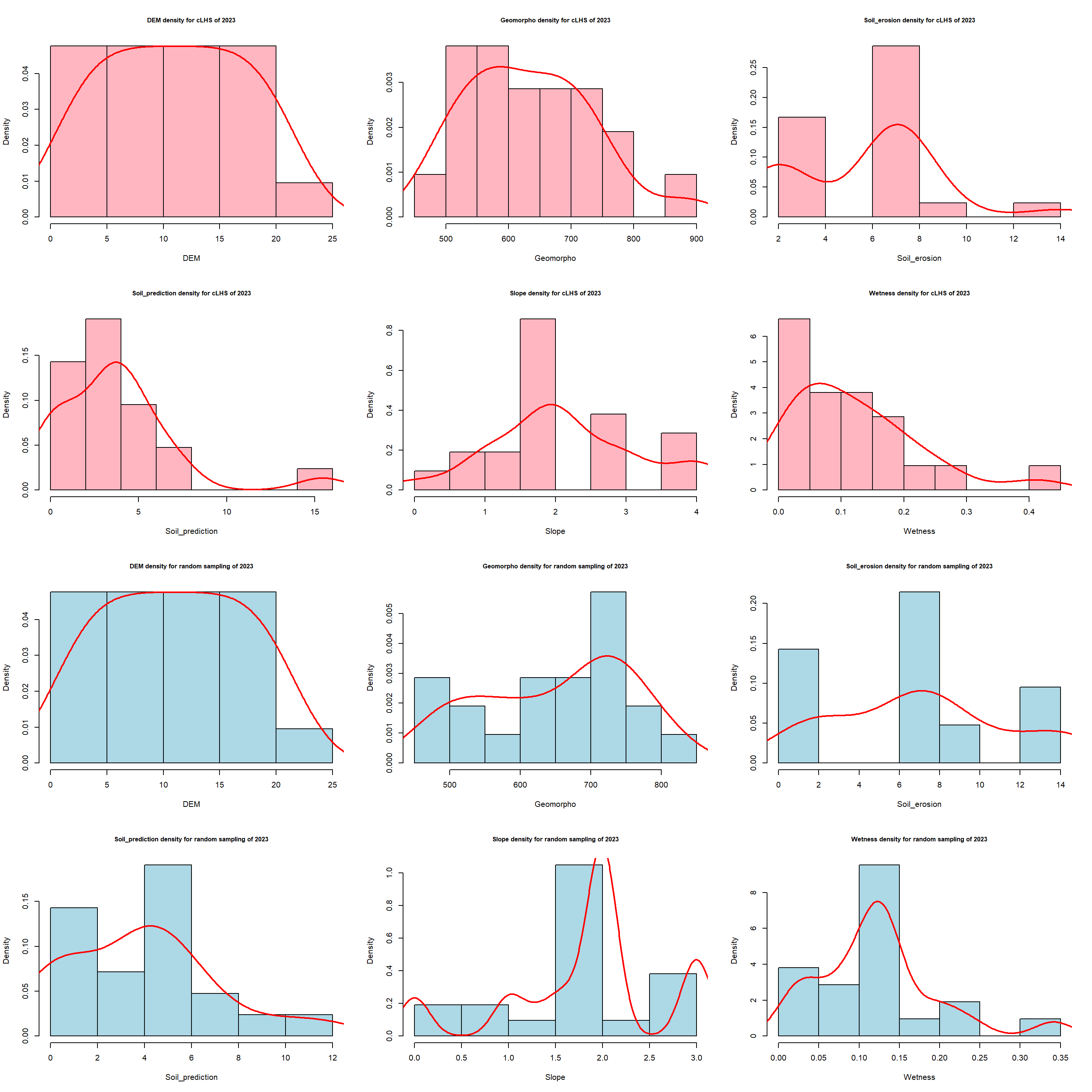
(#fig:density samples 2023)2023 Campaign samples distribution.