7 Digital soil mapping
7.1 Introduction
7.1.1 Purpose
We present here the methodology for the digital soil mapping based on the soil values from the spectra prediction.
7.1.2 Covariates
We used a set of 85 covariates mainly based on Zolfaghari Nia et al. (2022). All the data listed below are available freely online excepted for the digitized maps (geology, geohydrology and geomorphology).
| Name/ID | Original resolution (m) | Type/Unit |
|---|---|---|
| Landsat 8 Blue/LA.1 | 30 | 0.45 - 0.51 µm |
| Landsat 8 Green/LA.2 | 30 | 0.53 - 0.59 µm |
| Landsat 8 NDVI/LA.3 | 30 | - |
| Landsat 8 NDWI/LA.4 | 30 | - |
| Landsat 8 NIR/LA.5 | 30 | 0.85 - 0.88 µm |
| Landsat 8 Panchromatic/LA.6 | 15 | 0.52 - 0.90 µm |
| Landsat 8 Red/LA.7 | 30 | 0.64 - 0.67 µm |
| Landsat 8 SWIR1/LA.8 | 30 | 1.57 - 1.65 µm |
| Landsat 8 SWIR2/LA.9 | 30 | 2.11 - 2.29 µm |
| Landsat 8 EVI/LA.10 | 30 | - |
| Landsat 8 SAVI/LA.11 | 30 | - |
| Landsat 8 NDMI/LA.12 | 30 | - |
| Landsat 8 CORSI/LA.13 | 30 | - |
| Landsat 8 Brightness index/LA.14 | 30 | - |
| Landsat 8 Clay index/LA.15 | 30 | - |
| Landsat 8 Salinity index/LA.16 | 30 | - |
| Landsat 8 Carbonate index/LA.17 | 30 | - |
| Landsat 8 Gypsum index/LA.18 | 30 | - |
| MODIS EVI/MO.1 | 300 | - |
| MODIS LST day/MO.2 | 1000 | °C |
| MODIS LST night/MO.2 | 1000 | °C |
| MODIS NDVI/MO.4 | 300 | - |
| MODIS NIR/MO.5 | 300 | 0.841 - 0.876 µm |
| MODIS Red/MO.6 | 300 | 0.62 - 0.67 µm |
| MODIS SAVI/MO.7 | 300 | Meters |
| MODIS Brightness index/MO.8 | 300 | 35 classes |
| Distance rivers/OT.1 | 30 | 17 classes |
| Geology/OT.2 | 1 : 300 000 | 11 classes |
| Geomorphology/OT.3 | 1 : 300 000 | mm |
| Landuses/OT.4 | 10 | mm |
| PET sum/OT.5 | 750 | Kj m\(^{-2}\) |
| Prec. sum/OT.6 | 1000 | °C |
| SRAD sum/OT.7 | 1000 | m s\(^{-1}\) |
| Diff Max. Min. Temp./OT.8 | 1000 | 0.492 - 0.496 µm |
| Wind sum/OT.9 | 1000 | 0.559 - 0.560 µm |
| Sentinel 2 Blue/SE.1 | 10 | - |
| Sentinel 2 Green/SE.2 | 10 | - |
| Sentinel 2 NDVI/SE.3 | 20 | 0.833 - 0.835 µm |
| Sentinel 2 NDWI/SE.4 | 20 | 0.665 - 0.664 µm |
| Sentinel 2 NIR/SE.5 | 10 | 0.738 - 0.739 µm |
| Sentinel 2 Red/SE.6 | 10 | 0.739 - 0.740 µm |
| Sentinel 2 RedEdge1/SE.7 | 20 | 0.779 - 0.782 µm |
| Sentinel 2 RedEdge2/SE.8 | 20 | 1.610 - 1.613 µm |
| Sentinel 2 RedEdge3/SE.9 | 20 | 2.185 - 2.202 µm |
| Sentinel 2 SWIR1/SE.10 | 20 | 0.943 - 0.945 µm |
| Sentinel 2 SWIR2/SE.11 | 20 | - |
| Sentinel 2 water vapor/SE.12 | 90 | - |
| Sentinel 2 EVI/SE.13 | 20 | - |
| Sentinel 2 TVI/SE.14 | 20 | - |
| Sentinel 2 SAVI/SE.15 | 20 | - |
| Sentinel 2 LSWI/SE.16 | 20 | - |
| Sentinel 2 Clay index/SE.17 | 20 | - |
| Sentinel 2 Brightness index/SE.18 | 20 | - |
| Sentinel 2 Salinity index/SE.19 | 20 | - |
| Sentinel 2 Carbonate index/SE.20 | 20 | Radians |
| Sentinel 2 Gypsum index/SE.21 | 20 | - |
| Aspect/TE.1 | 30 | - |
| Channel network base level/TE.2 | 30 | - |
| Channel network distance/TE.3 | 30 | Meters |
| Connexity/TE.4 | 30 | - |
| DEM/TE.5 | 30 | - |
| Flow accumaltion/TE.6 | 30 | - |
| General curvature/TE.7 | 30 | - |
| MrRTF/TE.8 | 30 | Radians |
| MrVBF/TE.9 | 30 | - |
| Negative openness/TE.10 | 30 | - |
| Normalized height/TE.11 | 30 | Radians |
| Plan curvature/TE.12 | 30 | - |
| Positive openness/TE.13 | 30 | - |
| Profile curvature/TE.14 | 30 | Radians |
| Slope height/TE.15 | 30 | - |
| Slope/TE.16 | 30 | - |
| Standardized height/TE.17 | 30 | - |
| Surface landform/TE.18 | 30 | - |
| Terrain ruggedness index/TE.19 | 30 | - |
| Terrain texture/TE.20 | 30 | - |
| TPI/TE.21 | 30 | - |
| TWI/TE.22 | 30 | - |
| Total catchment area/TE.23 | 30 | 0.45 - 0.51 µm |
| Valley depth/TE.24 | 30 | 0.53 - 0.59 µm |
We create an Python API to access the Google Earth Engine plateforme. You can read to the ‘ipynb’ file for more info.
import ee
import geemap
import rasterio
from rasterio.features import shapes
import geopandas as gpd
from shapely.geometry import mapping
from shapely.geometry import shape
import os
from pydrive.auth import GoogleAuth
from pydrive.drive import GoogleDrive

ee.Authenticate()
ee.Initialize()

# Local file
raster_path = r".\data\Large_grid.tif"
with rasterio.open(raster_path) as src:
    image = src.read(1)
    mask = image > 0
    results = (
        {'properties': {'value': v}, 'geometry': s}
        for i, (s, v) in enumerate(
            shapes(image, mask=mask, transform=src.transform))
    )

# Convert in GeoDataFrame
geoms = list(results)
gdf = gpd.GeoDataFrame.from_features(geoms)

# Create a polygon and gee object
aoi_poly = gdf.union_all()
aoi = ee.Geometry(mapping(aoi_poly))

Map = geemap.Map()
Map.centerObject(aoi, 8)
Map.addLayer(aoi, {}, "AOI")
Map

def maskS2clouds(image):
    qa = image.select('QA60')
    cloudBitMask = 1 << 10
    cirrusBitMask = 1 << 11
    mask = qa.bitwiseAnd(cloudBitMask).eq(0).And(
        qa.bitwiseAnd(cirrusBitMask).eq(0))
    return image.updateMask(mask).divide(10000)

dataset = (
    ee.ImageCollection("COPERNICUS/S2_SR_HARMONIZED")
    .filterDate("2021-01-01", "2022-01-31")  # period
    .filter(ee.Filter.lt("CLOUDY_PIXEL_PERCENTAGE", 20))  # cloud < 20%
    .map(maskS2clouds)
)

# Median
S2_composite = dataset.median().clip(aoi)

def maskL8clouds(image):
    qa = image.select('QA_PIXEL')

    cloudBit        = 1 << 3
    cloudShadowBit  = 1 << 4
    # Cirrus have not been considered as it provides only black cells
    # cirrusConfMask  = 1 << 14

    mask = (qa.bitwiseAnd(cloudBit).eq(0)
            .And(qa.bitwiseAnd(cloudShadowBit).eq(0)))
    return image.updateMask(mask)


dataset = (
    ee.ImageCollection("LANDSAT/LC08/C02/T1_TOA")
    .filterDate("2021-01-01", "2022-01-01")  # period
    .map(maskL8clouds)
)

# Median
L8_composite = dataset.median().clip(aoi)

modisLST = ee.ImageCollection("MODIS/061/MOD11A2")
modisLSTFiltered = modisLST.filterDate("2021-01-01", "2022-01-31").filterBounds(aoi)
modisrefl = ee.ImageCollection('MODIS/061/MOD09Q1')
modisreflFiltered = modisrefl.filterDate("2021-01-01", "2022-01-31").filterBounds(aoi)
modisvege = ee.ImageCollection("MODIS/061/MOD13Q1")
modisvegeFiltered = modisvege.filterDate("2021-01-01", "2022-01-31").filterBounds(aoi)

def kelvin_to_celsius(image):
    return image.multiply(0.02).subtract(273.15).rename('LST_Celsius')

lstDay = modisLSTFiltered.select('LST_Day_1km').map(kelvin_to_celsius)
lstDayMedian = lstDay.median().clip(aoi)

lstNight = modisLSTFiltered.select('LST_Night_1km').map(kelvin_to_celsius)
lstNightMedian = lstNight.median().clip(aoi)

redBand = modisreflFiltered.select('sur_refl_b01').median().clip(aoi)
nirBand = modisreflFiltered.select('sur_refl_b02').median().clip(aoi)
NDVIBand = modisvegeFiltered.select('NDVI').median().clip(aoi)
EVIBand = modisvegeFiltered.select('EVI').median().clip(aoi)

# PET
et_monthly = ee.ImageCollection("projects/sat-io/open-datasets/global_et0/global_et0_monthly")

# Select all the months
months = ['et0_V3_01','et0_V3_02','et0_V3_03','et0_V3_04','et0_V3_05','et0_V3_06','et0_V3_07','et0_V3_08',
          'et0_V3_09','et0_V3_10','et0_V3_11','et0_V3_12']
subset = et_monthly.filter(ee.Filter.inList('system:index', months))

# Sum of PET
pet_select = subset.sum().rename('ET0_sum').clip(aoi)

# DEM
dem = ee.ImageCollection("COPERNICUS/DEM/GLO30").select("DEM").mosaic().clip(aoi)

Landuse = ee.ImageCollection('ESA/WorldCover/v200').first().clip(aoi)

geemap.ee_export_image(
    Landuse,
    filename=r".\data\Others\Landuse_raw.tif",
    scale=30,
    region=aoi,
    crs="EPSG:32638"
)

geemap.ee_export_image(
    pet_select,
    filename=r".\data\Others\PET_raw.tif",
    scale=800,
    region=aoi,
    crs="EPSG:32638"
)

geemap.ee_export_image(
    lstDayMedian,
    filename=r".\data\MODIS\MODIS_LST_day_raw.tif",
    scale=1000,
    region=aoi,
    crs="EPSG:32638"
)

geemap.ee_export_image(
    lstNightMedian,
    filename=r".\data\MODIS\MODIS_LST_night_raw.tif",
    scale=1000,
    region=aoi,
    crs="EPSG:32638"
)

geemap.ee_export_image(
    redBand,
    filename=r".\data\MODIS\MODIS_Red_raw.tif",
    scale=250,
    region=aoi,
    crs="EPSG:32638"
)

geemap.ee_export_image(
    nirBand,
    filename=r".\data\MODIS\MODIS_NIR_raw.tif",
    scale=250,
    region=aoi,
    crs="EPSG:32638"
)

geemap.ee_export_image(
    NDVIBand,
    filename=r".\data\MODIS\MODIS_NDVI_raw.tif",
    scale=250,
    region=aoi,
    crs="EPSG:32638"
)

geemap.ee_export_image(
    EVIBand,
    filename=r".\data\MODIS\MODIS_EVI_raw.tif",
    scale=250,
    region=aoi,
    crs="EPSG:32638"
)

task = ee.batch.Export.image.toDrive(
        image=dem,
        description = f"DEM_raw",
        scale = 30,
        region = aoi,
        crs = 'EPSG:32638',
        folder = 'GoogleEarthEngine',
        maxPixels = 1e13
    )
task.start()

S2_bands = ['B2', 'B3', 'B4', 'B5', 'B6', 'B7', 'B8', 'B9', 'B11', 'B12']

for band in S2_bands:
    task = ee.batch.Export.image.toDrive(
        image=S2_composite.select([band]),
        description = f"Sentinel2_{band}_2021_MedianComposite",
        scale = 30,
        region = aoi,
        crs = 'EPSG:32638',
        folder = 'GoogleEarthEngine',
        maxPixels = 1e13
    )
    task.start()

L8_bands = ['B2', 'B3', 'B4', 'B5', 'B6', 'B7', 'B8']

for band in L8_bands:
    task = ee.batch.Export.image.toDrive(
        image=L8_composite.select([band]),
        description = f"Landsat8_{band}_2021_MedianComposite",
        scale = 30,
        region = aoi,
        crs = 'EPSG:32638',
        folder = 'GoogleEarthEngine',
        maxPixels = 1e13
    )
    task.start()
7.1.2.1 Terrain
For the DEM and all the derivatives, we used SAGA GIS 9.3.1 software and all the specificties of the batch process are detailed below. The last LS factor corresponds to the Total catchment area covariate.
[2025-09-24/01:09:32] [Fill Sinks (Wang & Liu)] Execution started...
__________
[Fill Sinks (Wang & Liu)] Parameters:
Grid System: 30; 2840x 2175y; 258795x 4063035y
DEM: DEM_raw
Filled DEM: Filled DEM
Flow Directions: Flow Directions
Watershed Basins: Watershed Basins
Minimum Slope [Degree]: 0.1

__________
total execution time: 7000 milliseconds (07s)

[2025-09-24/01:09:39] [Fill Sinks (Wang & Liu)] Execution succeeded (07s)

[2025-09-24/01:18:18] [Simple Filter] Execution started...
__________
[Simple Filter] Parameters:
Grid System: 30; 2840x 2175y; 258795x 4063035y
Grid: DEM_raw [no sinks]
Filtered Grid: Filtered Grid
Filter: Smooth
Kernel Type: Square
Radius: 3

__________
total execution time: 3000 milliseconds (03s)

[2025-09-24/01:18:21] [Simple Filter] Execution succeeded (03s)

[2025-09-24/01:21:25] [Slope, Aspect, Curvature] Execution started...
__________
[Slope, Aspect, Curvature] Parameters:
Grid System: 30; 2840x 2175y; 258795x 4063035y
Elevation: DEM_raw [no sinks] [Smoothed]
Slope: Slope
Aspect: Aspect
Northness: <not set>
Eastness: <not set>
General Curvature: General Curvature
Profile Curvature: Profile Curvature
Plan Curvature: Plan Curvature
Tangential Curvature: <not set>
Longitudinal Curvature: <not set>
Cross-Sectional Curvature: <not set>
Minimal Curvature: <not set>
Maximal Curvature: <not set>
Total Curvature: <not set>
Flow Line Curvature: <not set>
Method: 9 parameter 2nd order polynom (Zevenbergen & Thorne 1987)
Unit: radians
Unit: radians

__________
total execution time: 1000 milliseconds (01s)

[2025-09-24/01:21:27] [Slope, Aspect, Curvature] Execution succeeded (01s)

[2025-09-24/16:21:11] [Channel Network and Drainage Basins] Execution started...
__________
[Channel Network and Drainage Basins] Parameters:
Grid System: 30; 2641x 1940y; 262905x 4067505y
Elevation: DEM [no sinks] [Smoothed]
Flow Direction: Flow Direction
Flow Connectivity: <not set>
Strahler Order: <not set>
Drainage Basins: Drainage Basins
Channels: Channels
Drainage Basins: Drainage Basins
Junctions: <not set>
Threshold: 5
Subbasins: false

__________
[Vectorizing Grid Classes] Parameters:
Grid System: 30; 2641x 1940y; 262905x 4067505y
Grid: Drainage Basins
Polygons: Polygons
Class Selection: all classes
Vectorised class as...: one single (multi-)polygon object
Keep Vertices on Straight Lines: false

[Vectorizing Grid Classes] execution time: 05s
__________
total execution time: 9000 milliseconds (09s)

[2025-09-24/16:21:20] [Channel Network and Drainage Basins] Execution succeeded (09s)

[2025-09-24/01:26:59] [Channel Network] Execution started...
__________
[Channel Network] Parameters:
Grid System: 30; 2840x 2175y; 258795x 4063035y
Elevation: DEM_raw [no sinks] [Smoothed]
Flow Direction: Flow Direction
Channel Network: Channel Network
Channel Direction: Channel Direction
Channel Network: Channel Network
Initiation Grid: DEM_raw [no sinks] [Smoothed]
Initiation Type: Greater than
Initiation Threshold: 0
Divergence: <not set>
Tracing: Max. Divergence: 5
Tracing: Weight: <not set>
Min. Segment Length: 10

__________
total execution time: 142000 milliseconds (02m 22s)

[2025-09-24/01:29:21] [Channel Network] Execution succeeded (02m 22s)

[2025-09-24/01:30:53] [Multiresolution Index of Valley Bottom Flatness (MRVBF)] Execution started...
__________
[Multiresolution Index of Valley Bottom Flatness (MRVBF)] Parameters:
Grid System: 30; 2840x 2175y; 258795x 4063035y
Elevation: DEM_raw [no sinks] [Smoothed]
MRVBF: MRVBF
MRRTF: MRRTF
Initial Threshold for Slope: 16
Threshold for Elevation Percentile (Lowness): 0.4
Threshold for Elevation Percentile (Upness): 0.35
Shape Parameter for Slope: 4
Shape Parameter for Elevation Percentile: 3
Update Views: true
Classify: false
Maximum Resolution (Percentage): 100

step: 1, resolution: 30.00, threshold slope 16.00
step: 2, resolution: 30.00, threshold slope 8.00
step: 3, resolution: 90.00, threshold slope 4.00
step: 4, resolution: 270.00, threshold slope 2.00
step: 5, resolution: 810.00, threshold slope 1.00
step: 6, resolution: 2430.00, threshold slope 0.50
step: 7, resolution: 7290.00, threshold slope 0.25
step: 8, resolution: 21870.00, threshold slope 0.12
step: 9, resolution: 65610.00, threshold slope 0.06
step: 10, resolution: 196830.00, threshold slope 0.03
__________
total execution time: 105000 milliseconds (01m 45s)

[2025-09-24/01:32:38] [Multiresolution Index of Valley Bottom Flatness (MRVBF)] Execution succeeded (01m 45s)

[2025-09-24/01:33:26] [Topographic Openness] Execution started...
__________
[Topographic Openness] Parameters:
Grid System: 30; 2840x 2175y; 258795x 4063035y
Elevation: DEM_raw [no sinks] [Smoothed]
Positive Openness: Positive Openness
Negative Openness: Negative Openness
Radial Limit: 10000
Directions: all
Number of Sectors: 8
Method: line tracing
Unit: Radians
Difference from Nadir: true

__________
total execution time: 101000 milliseconds (01m 41s)

[2025-09-24/01:35:07] [Topographic Openness] Execution succeeded (01m 41s)

[2025-09-24/02:11:27] [Vertical Distance to Channel Network] Execution started...
__________
[Vertical Distance to Channel Network] Parameters:
Grid System: 30; 2840x 2175y; 258795x 4063035y
Elevation: DEM_raw [no sinks] [Smoothed]
Channel Network: Channel Network
Vertical Distance to Channel Network: Vertical Distance to Channel Network
Channel Network Base Level: Channel Network Base Level
Tension Threshold: 1
Maximum Iterations: 0
Keep Base Level below Surface: true

Level: 12; Iterations: 1; Maximum change: 0.000000
Level: 11; Iterations: 1; Maximum change: 0.000000
Level: 10; Iterations: 1; Maximum change: 0.000000
Level: 9; Iterations: 1; Maximum change: 0.000000
Level: 8; Iterations: 1; Maximum change: 0.000000
Level: 7; Iterations: 1; Maximum change: 0.000000
Level: 6; Iterations: 1; Maximum change: 0.000000
Level: 5; Iterations: 1; Maximum change: 0.000000
Level: 4; Iterations: 4; Maximum change: 0.354675
Level: 3; Iterations: 6; Maximum change: 0.844788
Level: 2; Iterations: 15; Maximum change: 0.925110
Level: 1; Iterations: 20; Maximum change: 0.932373
__________
total execution time: 13000 milliseconds (13s)

[2025-09-24/02:11:40] [Vertical Distance to Channel Network] Execution succeeded (13s)

[2025-09-24/01:38:34] [Terrain Surface Convexity] Execution started...
__________
[Terrain Surface Convexity] Parameters:
Grid System: 30; 2840x 2175y; 258795x 4063035y
Elevation: DEM_raw [no sinks] [Smoothed]
Convexity: Convexity
Laplacian Filter Kernel: conventional four-neighbourhood
Type: convexity
Flat Area Threshold: 0
Scale (Cells): 10
Method: resampling
Weighting Function: gaussian
Bandwidth: 0.7

__________
total execution time: 1000 milliseconds (01s)

[2025-09-24/01:38:35] [Terrain Surface Convexity] Execution succeeded (01s)

[2025-09-24/16:53:51] [Flow Accumulation (One Step)] Execution started...
__________
[Flow Accumulation (One Step)] Parameters:
Elevation: DEM [no sinks] [Smoothed]
Flow Accumulation: Flow Accumulation
Specific Catchment Area: Specific Catchment Area
Preprocessing: Fill Sinks (Wang & Liu)
Flow Routing: Deterministic Infinity

__________
[Fill Sinks XXL (Wang & Liu)] Parameters:
Grid System: 30; 2641x 1940y; 262905x 4067505y
DEM: DEM [no sinks] [Smoothed]
Filled DEM: Filled DEM
Minimum Slope [Degree]: 0.0001

[Fill Sinks XXL (Wang & Liu)] execution time: 03s
__________
[Flow Accumulation (Top-Down)] Parameters:
Grid System: 30; 2641x 1940y; 262905x 4067505y
Elevation: DEM [no sinks] [Smoothed] [no sinks]
Sink Routes: <not set>
Weights: <not set>
Flow Accumulation: Flow Accumulation
Input for Mean over Catchment: <not set>
Material for Accumulation: <not set>
Step: 1
Flow Accumulation Unit: cell area
Flow Path Length: <not set>
Channel Direction: <not set>
Method: Deterministic Infinity
Thresholded Linear Flow: false

[Flow Accumulation (Top-Down)] execution time: 07s
__________
[Flow Width and Specific Catchment Area] Parameters:
Grid System: 30; 2641x 1940y; 262905x 4067505y
Elevation: DEM [no sinks] [Smoothed] [no sinks]
Flow Width: Flow Width
Total Catchment Area (TCA): Flow Accumulation
Specific Catchment Area (SCA): Specific Catchment Area (SCA)
Coordinate Unit: meter
Method: Aspect

[Flow Width and Specific Catchment Area] execution time: 01s
__________
total execution time: 11000 milliseconds (11s)

[2025-09-24/16:54:02] [Flow Accumulation (One Step)] Execution succeeded (11s)

[2025-09-24/01:41:22] [Relative Heights and Slope Positions] Execution started...
__________
[Relative Heights and Slope Positions] Parameters:
Grid System: 30; 2840x 2175y; 258795x 4063035y
Elevation: DEM_raw [no sinks] [Smoothed]
Slope Height: Slope Height
Valley Depth: Valley Depth
Normalized Height: Normalized Height
Standardized Height: Standardized Height
Mid-Slope Position: Mid-Slope Position
w: 0.5
t: 10
e: 2

[2025-09-24/01:41:22] Pass 1
[2025-09-24/01:42:51] Pass 2
__________
total execution time: 214000 milliseconds (03m 34s)

[2025-09-24/01:44:56] [Relative Heights and Slope Positions] Execution succeeded (03m 34s)

[2025-09-24/01:45:50] [TPI Based Landform Classification] Execution started...
__________
[TPI Based Landform Classification] Parameters:
Grid System: 30; 2840x 2175y; 258795x 4063035y
Elevation: DEM_raw [no sinks] [Smoothed]
Landforms: Landforms
Small Scale: 0; 100
Large Scale: 0; 1000
Weighting Function: no distance weighting

__________
[Topographic Position Index (TPI)] Parameters:
Grid System: 30; 2840x 2175y; 258795x 4063035y
Elevation: DEM_raw [no sinks] [Smoothed]
Topographic Position Index: Topographic Position Index
Standardize: true
Scale: 0; 100
Weighting Function: no distance weighting

[Topographic Position Index (TPI)] execution time: 02s
__________
[Topographic Position Index (TPI)] Parameters:
Grid System: 30; 2840x 2175y; 258795x 4063035y
Elevation: DEM_raw [no sinks] [Smoothed]
Topographic Position Index: Topographic Position Index
Standardize: true
Scale: 0; 1000
Weighting Function: no distance weighting

[Topographic Position Index (TPI)] execution time: 03m 51s
__________
total execution time: 234000 milliseconds (03m 54s)

[2025-09-24/01:49:44] [TPI Based Landform Classification] Execution succeeded (03m 54s)

[2025-09-24/01:51:16] [Topographic Position Index (TPI)] Execution started...
__________
[Topographic Position Index (TPI)] Parameters:
Grid System: 30; 2840x 2175y; 258795x 4063035y
Elevation: DEM_raw [no sinks] [Smoothed]
Topographic Position Index: Topographic Position Index
Standardize: true
Scale: 0; 100
Weighting Function: no distance weighting

__________
total execution time: 3000 milliseconds (03s)

[2025-09-24/01:51:19] [Topographic Position Index (TPI)] Execution succeeded (03s)

[2025-09-24/01:51:58] [Terrain Surface Texture] Execution started...
__________
[Terrain Surface Texture] Parameters:
Grid System: 30; 2840x 2175y; 258795x 4063035y
Elevation: DEM_raw [no sinks] [Smoothed]
Texture: Texture
Flat Area Threshold: 1
Scale (Cells): 10
Method: resampling
Weighting Function: gaussian
Bandwidth: 0.7

__________
total execution time: 4000 milliseconds (04s)

[2025-09-24/01:52:02] [Terrain Surface Texture] Execution succeeded (04s)

[2025-09-24/17:05:39] [Terrain Ruggedness Index (TRI)] Execution started...
__________
[Terrain Ruggedness Index (TRI)] Parameters:
Grid System: 30; 2641x 1940y; 262905x 4067505y
Elevation: DEM [no sinks] [Smoothed]
Terrain Ruggedness Index (TRI): Terrain Ruggedness Index (TRI)
Search Mode: Square
Search Radius: 3
Weighting Function: no distance weighting

__________
total execution time: 2000 milliseconds (02s)

[2025-09-24/17:05:41] [Terrain Ruggedness Index (TRI)] Execution succeeded (02s)

[2025-09-24/17:08:48] [Topographic Wetness Index (One Step)] Execution started...
__________
[Topographic Wetness Index (One Step)] Parameters:
Elevation: DEM [no sinks] [Smoothed]
Topographic Wetness Index: Topographic Wetness Index
Flow Distribution: Deterministic Infinity

__________
[Sink Removal] Parameters:
Grid System: 30; 2641x 1940y; 262905x 4067505y
DEM: DEM [no sinks] [Smoothed]
Sink Route: <not set>
Preprocessed DEM: Preprocessed DEM
Method: Fill Sinks
Threshold: false
Epsilon: 0.001

number of processed sinks: 2266
[Sink Removal] execution time: 13s
__________
[Flow Accumulation (Top-Down)] Parameters:
Grid System: 30; 2641x 1940y; 262905x 4067505y
Elevation: DEM [no sinks] [Smoothed] [no sinks]
Sink Routes: <not set>
Weights: <not set>
Flow Accumulation: Flow Accumulation
Input for Mean over Catchment: <not set>
Material for Accumulation: <not set>
Step: 1
Flow Accumulation Unit: cell area
Flow Path Length: <not set>
Channel Direction: <not set>
Method: Deterministic Infinity
Thresholded Linear Flow: false

[Flow Accumulation (Top-Down)] execution time: 06s
__________
[Flow Width and Specific Catchment Area] Parameters:
Grid System: 30; 2641x 1940y; 262905x 4067505y
Elevation: DEM [no sinks] [Smoothed] [no sinks]
Flow Width: Flow Width
Total Catchment Area (TCA): Flow Accumulation
Specific Catchment Area (SCA): Specific Catchment Area (SCA)
Coordinate Unit: meter
Method: Aspect

[Flow Width and Specific Catchment Area] execution time: 01s
__________
[Slope, Aspect, Curvature] Parameters:
Grid System: 30; 2641x 1940y; 262905x 4067505y
Elevation: DEM [no sinks] [Smoothed] [no sinks]
Slope: Slope
Aspect: <not set>
Northness: <not set>
Eastness: <not set>
General Curvature: <not set>
Profile Curvature: <not set>
Plan Curvature: <not set>
Tangential Curvature: <not set>
Longitudinal Curvature: <not set>
Cross-Sectional Curvature: <not set>
Minimal Curvature: <not set>
Maximal Curvature: <not set>
Total Curvature: <not set>
Flow Line Curvature: <not set>
Method: 9 parameter 2nd order polynom (Zevenbergen & Thorne 1987)
Unit: radians
Unit: radians

[Slope, Aspect, Curvature] execution time: 01s
__________
[Topographic Wetness Index] Parameters:
Grid System: 30; 2641x 1940y; 262905x 4067505y
Slope: Slope
Catchment Area: Specific Catchment Area (SCA)
Transmissivity: <not set>
Topographic Wetness Index: Topographic Wetness Index
Area Conversion: no conversion (areas already given as specific catchment area)
Method (TWI): Standard

[Topographic Wetness Index] execution time: less than 1 millisecond
__________
total execution time: 22000 milliseconds (22s)

[2025-09-24/17:09:11] [Topographic Wetness Index (One Step)] Execution succeeded (22s)

[2025-09-24/01:58:44] [LS Factor (One Step)] Execution started...
__________
[LS Factor (One Step)] Parameters:
DEM: DEM_raw [no sinks] [Smoothed]
LS Factor: LS Factor
Feet Conversion: false
Method: Moore et al. 1991
Preprocessing: none
Minimum Slope: 0.0001

__________
[Slope, Aspect, Curvature] Parameters:
Grid System: 30; 2840x 2175y; 258795x 4063035y
Elevation: DEM_raw [no sinks] [Smoothed]
Slope: Slope
Aspect: <not set>
Northness: <not set>
Eastness: <not set>
General Curvature: <not set>
Profile Curvature: <not set>
Plan Curvature: <not set>
Tangential Curvature: <not set>
Longitudinal Curvature: <not set>
Cross-Sectional Curvature: <not set>
Minimal Curvature: <not set>
Maximal Curvature: <not set>
Total Curvature: <not set>
Flow Line Curvature: <not set>
Method: 9 parameter 2nd order polynom (Zevenbergen & Thorne 1987)
Unit: radians
Unit: radians

[Slope, Aspect, Curvature] execution time: 01s
__________
[Flow Accumulation (Top-Down)] Parameters:
Grid System: 30; 2840x 2175y; 258795x 4063035y
Elevation: DEM_raw [no sinks] [Smoothed]
Sink Routes: <not set>
Weights: <not set>
Flow Accumulation: Flow Accumulation
Input for Mean over Catchment: <not set>
Material for Accumulation: <not set>
Step: 1
Flow Accumulation Unit: cell area
Flow Path Length: <not set>
Channel Direction: <not set>
Method: Multiple Flow Direction
Thresholded Linear Flow: false
Convergence: 1.1
Contour Length: false

[Flow Accumulation (Top-Down)] execution time: 04s
__________
[Flow Width and Specific Catchment Area] Parameters:
Grid System: 30; 2840x 2175y; 258795x 4063035y
Elevation: DEM_raw [no sinks] [Smoothed]
Flow Width: Flow Width
Total Catchment Area (TCA): Flow Accumulation
Specific Catchment Area (SCA): Specific Catchment Area (SCA)
Coordinate Unit: meter
Method: Aspect

[Flow Width and Specific Catchment Area] execution time: less than 1 millisecond
__________
[LS Factor] Parameters:
Grid System: 30; 2840x 2175y; 258795x 4063035y
Slope: Slope
Catchment Area: Specific Catchment Area (SCA)
LS Factor: LS Factor
Area to Length Conversion: no conversion (areas already given as specific catchment area)
Feet Adjustment: false
Method (LS): Moore et al. 1991
Rill/Interrill Erosivity: 1
Stability: stable

[LS Factor] execution time: less than 1 millisecond
__________
total execution time: 6000 milliseconds (06s)

[2025-09-24/01:58:50] [LS Factor (One Step)] Execution succeeded (06s)
7.1.2.2 Remote sensing images and indexes
The Landsat 8 images were collected via a Google Earth Engine script on a period covering 2020, the median of the composite image from Tier 1 TOA collection was used. The Sentinel 2 image were collected via a Google Earth Engine script on a period covering 2021, the median of the composite image from MultiSpectral Instrument Level-2A collection was used.The land surface temperature (LST) and other MODIS component were computed also on Google Earth with a time covering from 2020 to 2021. the median of the MODIS Terra collection was used. The javascript codes for scraping these images are available in the supplementary file inside the “7 - DSM/code” folder. We computed the following indexes: Normalized Difference Vegetation Index (NDVI); Normalized Difference Water Index (NDWI); Enhanced Vegetation Index (EVI); Soil Adjusted Vegetation Index (SAVI); Transformed Vegetation Index (TVI); Normilized Difference Moisture Index (NDMI); COmbined Specteral Response Index (COSRI); Land Surface Water Index (LSWI).
\[ NDVI = \frac{NIR - Red}{NIR + Red} \]
Rouse et al. (1974)
\[ NDWI = \frac{Green - NIR}{Green + NIR} \]
McFeeters (1996)
\[ EVI = G\frac{NIR - Red}{(NIR + 6Red - 7.5Blue) + L} \]
Where \(G\) is 2.5 and \(L\) is 1 A. Huete, Justice, and Liu (1994)
\[ SAVI = (1 + L)\frac{NIR - Red}{NIR + Red + L} \]
Where \(L\) is 0.5. A. R. Huete (1988)
\[ TVI = \sqrt{NDVI + 0.5} \]
Deering (1975)
\[ NDMI = \frac{NIR - SWIR1}{NIR + SWIR1} \]
Gao (1996)
\[ COSRI = \frac{Blue + Green}{Red + NIR} * NDVI \]
Fernández-Buces et al. (2006)
\[ LSWI = \frac{NIR - SWIR1}{NIR + SWIR1} \]
Chandrasekar et al. (2010)
\[ Brightness~index = \sqrt{Red^2 + NIR^2} \]
Khan et al. (2001)
\[ Simple~Ratio~Clay~index = \frac{SWIR1}{SWIR2} \]
Bousbih et al. (2019)
\[ Salinity~index = \frac{SWIR1 - SWIR2}{SWIR1 - NIR} \]
Also called NIR-SWIR index (NSI) Abuelgasim and Ammad (2019)
\[ Carbonate~index = \frac{Red}{Green} \]
Boettinger et al. (2008)
\[ Gypsum~index = \frac{SWIR1 - SWIR2}{SWIR1 + SWIR2} \]
Nield, Boettinger, and Ramsey (2007)
7.1.3 Soil properties
The soil 10 variables measurements for the five soil depth increment came from the predictions of the previous chapter and can be found online at: https://doi.org/10.1594/PANGAEA.973700.
7.1.4 Preparation of the data
All raster were sampled to 30 x 30 m tiles to match the DEM. We used bilinear method excepted for the discrete maps (geology and geomorphology) where we used ngb resampling. The heavier data from GEE were also called from the GoogleDrive and WorldClim directly collected from ‘geodata’ package. The the vector data were also transformed in raster beeing resampled.
# 0.1 Prepare environment ======================================================

# Folder check
getwd()

# Clean up workspace
rm(list = ls(all.names = TRUE))

# 0.2 Install packages =========================================================

install.packages("pacman")        #Install and load the "pacman" package (allow easier download of packages)
library(pacman)
pacman::p_load(pastclim, terra, sf, httr, geodata, googledrive, mapview) # Specify required packages and download it if needed

# 0.3 Show session infos =======================================================

sessionInfo()

# 01 Import data sets ##########################################################

# 01.1 Import background layers ================================================
grid <- rast("./data/Small_grid_UTM38.tif")
crs(grid) <- "EPSG:32638"

# 01.2 Import from Google Drive ================================================
drive_auth()
files <- drive_ls()

# Import Sentinel 2
file <- files[grepl("Sentinel2", files$name), ]
for (i in 1:nrow(file)) {
  drive_download(
    as_id(file$id[[i]]),
    path = paste0("./data/Sentinel/Raw_",file[[1]][[i]]),
    overwrite = TRUE)
}

# Import Landsat 8
file <- files[grepl("Landsat8", files$name), ]
for (i in 1:nrow(file)) {
  drive_download(
    as_id(file$id[[i]]),
    path = paste0("./data/Landsat/Raw_",file[[1]][[i]]),
    overwrite = TRUE)
}

file <- files[grepl("DEM", files$name), ]
drive_download(
  as_id(file$id),
  path = paste0("./data/Others/",file[[1]][[1]]),
  overwrite = TRUE)


# 03 Resize data ###############################################################

# 03.1 Resize GEE single data ==================================================
DEM_raw <- rast("./data/Others/DEM_raw.tif")
PET_raw <- rast("./data/Others/PET_raw.tif")
Landuse_raw <- rast("./data/Others/Landuse_raw.tif")
EVI_raw <- rast("./data/MODIS/MODIS_EVI_raw.tif")
NDVI_raw <- rast("./data/MODIS/MODIS_NDVI_raw.tif")
NIR_raw <- rast("./data/MODIS/MODIS_NIR_raw.tif")
Red_raw <- rast("./data/MODIS/MODIS_Red_raw.tif")
LST_day_raw <- rast("./data/MODIS/MODIS_LST_day_raw.tif")
LST_night_raw <- rast("./data/MODIS/MODIS_LST_night_raw.tif")

DEM <- crop(DEM_raw, grid)

PET <- resample(PET_raw, DEM, method = "bilinear")
PET <- crop(PET, DEM)
Landuse <- resample(Landuse_raw, DEM, method = "mode")
Landuse <- crop(Landuse, DEM)
EVI <- resample(EVI_raw, DEM, method = "bilinear")
EVI <- crop(EVI, DEM)
NDVI <- resample(NDVI_raw, DEM, method = "bilinear")
NDVI <- crop(NDVI, DEM)
NIR <- resample(NIR_raw, DEM, method = "bilinear")
NIR <- crop(NIR, DEM)
Red <- resample(Red_raw, DEM, method = "bilinear")
Red <- crop(Red, DEM)
LST_day <- resample(LST_day_raw, DEM, method = "bilinear")
LST_day <- crop(LST_day, DEM)
LST_night <- resample(LST_night_raw, DEM, method = "bilinear")
LST_night <- crop(LST_night, DEM)

writeRaster(DEM, "./data/Others/DEM.tif", overwrite=TRUE)
writeRaster(PET, "./data/Others/PET.tif", overwrite=TRUE)
writeRaster(Landuse, "./data/Others/Landuse.tif", overwrite=TRUE)
writeRaster(EVI, "./data/MODIS/MODIS_EVI.tif", overwrite=TRUE)
writeRaster(NDVI, "./data/MODIS/MODIS_NDVI.tif", overwrite=TRUE)
writeRaster(NIR, "./data/MODIS/MODIS_NIR.tif", overwrite=TRUE)
writeRaster(Red, "./data/MODIS/MODIS_Red.tif", overwrite=TRUE)
writeRaster(LST_day, "./data/MODIS/MODIS_LST_day.tif", overwrite=TRUE)
writeRaster(LST_night, "./data/MODIS/MODIS_LST_night.tif", overwrite=TRUE)

rm(list=setdiff(ls(), c("DEM", "grid")))

# 03.2 Resize GEE sentinel and landsat data ====================================

Sentinel <- rast(list.files("./data/Sentinel/", full.names = TRUE))
Sentinel_names <- list.files("./data/Sentinel/", full.names = FALSE)

patterns  <- c("B2", "B3", "B4", "B5", "B6", "B7", "B8", "B9", "B11", "B12")
replacers <- c("blue", "green", "red", "redEdge1", "redEdge2", "redEdge3", "NIR", "water", "SWIR1", "SWIR2")

for (i in seq_along(patterns)) {
  Sentinel_names <- gsub(patterns[i], replacers[i], Sentinel_names)
}
names(Sentinel) <- gsub("\\.tif$", "", Sentinel_names)
names(Sentinel) <- gsub("Raw_", "", names(Sentinel))

for (i in 1:nlyr(Sentinel)) {
  r <-resample(Sentinel[[i]], DEM, method = "bilinear")
  r <- crop(r, DEM)
  writeRaster(r, paste0("./data/Sentinel/",names(r),".tif"), overwrite=T)
}

Landsat <- rast(list.files("./data/Landsat/", full.names = TRUE))
Landsat_names <- list.files("./data/Landsat/", full.names = FALSE)

patterns  <- c("B2", "B3", "B4", "B5", "B6", "B7", "B8")
replacers <- c("blue", "green", "red", "NIR", "SWIR1", "SWIR2", "PAN")

for (i in seq_along(patterns)) {
  Landsat_names <- gsub(patterns[i], replacers[i], Landsat_names)
}
names(Landsat) <- gsub("\\.tif$", "", Landsat_names)
names(Landsat) <- gsub("Raw_", "", names(Landsat))

for (i in 1:nlyr(Landsat)) {
  r <-resample(Landsat[[i]], DEM, method = "bilinear")
  r <- crop(r, DEM)
  writeRaster(r, paste0("./data/Landsat/",names(r),".tif"), overwrite=T)
}

# 04 Download and compute the present-climate data #############################

# 04.1 Download the present WolrdClim  =========================================
temp.min <- worldclim_country("Iraq",var="tmin", res=0.5, "./data/WolrdClim.tif", version="2.1")
temp.max <- worldclim_country("Iraq",var="tmax", res=0.5, "./data/WolrdClim.tif", version="2.1")
prec <- worldclim_country("Iraq",var="prec", res=0.5, "./data/WolrdClim.tif", version="2.1")
srad <- worldclim_country("Iraq",var="srad", res=0.5, "./data/WolrdClim.tif", version="2.1")
wind <- worldclim_country("Iraq",var="wind", res=0.5, "./data/WolrdClim.tif", version="2.1")

# 04.2 Resize the present WolrdClim temperatures ===============================
temp.min_mean <- mean(temp.min)
temp.max_mean <- mean(temp.max)
BIO01 <- temp.max_mean - temp.min_mean
BIO01 <- project(BIO01, "EPSG:32638")
BIO01 <-resample(BIO01, DEM, method = "bilinear") #Careful to implement "near" option for classification maps
BIO01 <- crop(BIO01, DEM)
writeRaster(BIO01, "./data/Others/WorldClim_Temp.tif", overwrite=T)
plot(BIO01)

# 04.3 Resize the present WolrdClim precipiations ==============================
prec_sum <- sum(prec)
BIO12 <- project(prec_sum, "EPSG:32638")
BIO12 <-resample(BIO12, DEM, method = "bilinear") #Careful to implement "near" option for classification maps
BIO12 <-crop(BIO12, DEM)
writeRaster(BIO12, "./data/Others/WorldClim_Prec.tif", overwrite=T)
plot(BIO12)

# 04.4 Resize the present WolrdClim solar radiations ===========================
srad_sum <- sum(srad)
srad <- project(srad_sum, "EPSG:32638")
srad <-resample(srad, DEM, method = "bilinear") #Careful to implement "near" option for classification maps
srad <-crop(srad, DEM)
writeRaster(srad, "./data/Others/WorldClim_Srad.tif", overwrite=T)
plot(srad)

# 04.5 Resize the present WolrdClim wind forces ================================
wind_sum <- sum(wind)
wind <- project(wind_sum, "EPSG:32638")
wind <-resample(wind, DEM, method = "bilinear") #Careful to implement "near" option for classification maps
wind <-crop(wind, DEM)
writeRaster(wind, "./data/Others/WorldClim_Wind.tif", overwrite=T)
plot(wind)

# 05 Convert Shapefile data ####################################################

# 05.1 Convert from polylign to distance raster ================================
water <- st_read("./data/Natural.gpkg", layer = "Waterways")
mapview(water)

water_raster  <- rasterize(vect(water), DEM, field=1, background=NA)
dist_water <- distance(water_raster)

writeRaster(dist_water, "./data/Others/Distance to water.tif", overwrite=TRUE)

# 05.2 Convert from polygon to raster ==========================================

geomorpho <- st_read("./data/Natural.gpkg", layer = "Geomorphology")
geol <- st_read("./data/Natural.gpkg", layer = "Geology")

geomorpho_raster  <- rasterize(vect(geomorpho), DEM, field="Class", background=NA)
geol_raster  <- rasterize(vect(geol), DEM, field="Class", background=NA)

writeRaster(geomorpho_raster, "./data/Others/Geomorphology.tif", overwrite=TRUE)
writeRaster(geol_raster, "./data/Others/Geology.tif", overwrite=TRUE)
7.2 Soil digital mapping preparation
7.2.1 Preparation of the environment
# 0.1 Prepare environment ======================================================

# Folder check
getwd()

# Set folder direction
setwd()

# Clean up workspace
rm(list = ls(all.names = TRUE))

# 0.2 Install packages =========================================================

install.packages("pacman")        #Install and load the "pacman" package (allow easier download of packages)
library(pacman)

pacman::p_load(dplyr, tidyr,ggplot2, mapview, sf, cli, terra,  corrplot, doParallel, viridis, Boruta,  caret,
               quantregForest, readr, rpart, reshape2, usdm, soiltexture, compositions, patchwork)

# 0.3 Show session infos =======================================================
R version 4.5.1 (2025-06-13 ucrt)
Platform: x86_64-w64-mingw32/x64
Running under: Windows 11 x64 (build 26200)
Matrix products: default
LAPACK version 3.12.1
locale:
[1] LC_COLLATE=French_France.utf8 LC_CTYPE=French_France.utf8 LC_MONETARY=French_France.utf8 LC_NUMERIC=C
[5] LC_TIME=French_France.utf8
time zone: Europe/Paris
tzcode source: internal
attached base packages:
[1] parallel stats graphics grDevices utils datasets methods base
other attached packages:
[1] patchwork_1.3.2 compositions_2.0-9 soiltexture_1.5.3 usdm_2.1-7 reshape2_1.4.5 rpart_4.1.24
[7] readr_2.1.6 quantregForest_1.3-7.1 RColorBrewer_1.1-3 randomForest_4.7-1.2 caret_7.0-1 lattice_0.22-7
[13] Boruta_9.0.0 viridis_0.6.5 viridisLite_0.4.2 doParallel_1.0.17 iterators_1.0.14 foreach_1.5.2
[19] corrplot_0.95 terra_1.8-93 cli_3.6.5 sf_1.0-24 mapview_2.11.4 ggplot2_4.0.1
[25] tidyr_1.3.2 dplyr_1.1.4
loaded via a namespace (and not attached):
[1] DBI_1.2.3 pROC_1.19.0.1 gridExtra_2.3 tcltk_4.5.1 rlang_1.1.7 magrittr_2.0.4
[7] otel_0.2.0 e1071_1.7-17 compiler_4.5.1 png_0.1-8 vctrs_0.7.0 stringr_1.6.0
[13] pkgconfig_2.0.3 fastmap_1.2.0 leafem_0.2.5 rmarkdown_2.30 tzdb_0.5.0 prodlim_2025.04.28
[19] purrr_1.2.1 xfun_0.56 satellite_1.0.6 recipes_1.3.1 R6_2.6.1 stringi_1.8.7
[25] parallelly_1.46.1 lubridate_1.9.4 Rcpp_1.1.1 bookdown_0.46 knitr_1.51 future.apply_1.20.1
[31] base64enc_0.1-3 pacman_0.5.1 Matrix_1.7-4 splines_4.5.1 nnet_7.3-20 timechange_0.3.0
[37] tidyselect_1.2.1 rstudioapi_0.18.0 dichromat_2.0-0.1 yaml_2.3.12 timeDate_4051.111 codetools_0.2-20
[43] listenv_0.10.0 tibble_3.3.1 plyr_1.8.9 withr_3.0.2 S7_0.2.1 evaluate_1.0.5
[49] future_1.69.0 survival_3.8-6 bayesm_3.1-7 units_1.0-0 proxy_0.4-29 pillar_1.11.1
[55] tensorA_0.36.2.1 rsconnect_1.7.0 KernSmooth_2.23-26 stats4_4.5.1 generics_0.1.4 sp_2.2-0
[61] hms_1.1.4 scales_1.4.0 globals_0.18.0 class_7.3-23 glue_1.8.0 tools_4.5.1
[67] robustbase_0.99-6 data.table_1.18.0 ModelMetrics_1.2.2.2 gower_1.0.2 grid_4.5.1 crosstalk_1.2.2
[73] ipred_0.9-15 nlme_3.1-168 raster_3.6-32 lava_1.8.2 DEoptimR_1.1-4 gtable_0.3.6
[79] digest_0.6.39 classInt_0.4-11 htmlwidgets_1.6.4 farver_2.1.2 htmltools_0.5.9 lifecycle_1.0.5 7.2.2 Prepare the data
# 01 Import data sets ##########################################################
# 01.1 Import soils infos ======================================================
# From the data accessible at the https://doi.org/10.1594/PANGAEA.973700
soil_infos <- read.csv("./data/MIR_spectra_prediction.csv", sep=";")
soil_infos$Depth..bot <- as.factor(soil_infos$Depth..bot)
soil_infos <- soil_infos[,-c(5,7,8)]
soil_list <- split(soil_infos, soil_infos$Depth..bot)
depths <- c("0_10", "10_30", "30_50", "50_70", "70_100")
names(soil_list) <- depths
soil_infos <- soil_list
for (i in 1:length(soil_infos)) {
soil_infos[[i]] <- soil_infos[[i]][,-c(2,5)]
colnames(soil_infos[[i]]) <- c("Site_name","Latitude","Longitude","pH","CaCO3","Nt","Ct","Corg","EC","Sand","Silt","Clay","MWD")
write.csv(soil_infos[[i]], paste0("./data/Infos_",names(soil_infos[i]),"_soil.csv"))
}
# Histogramm ploting with normal and sqrt values
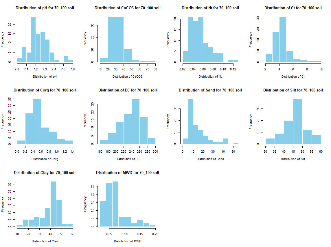
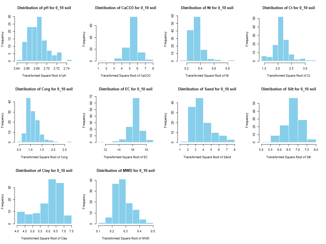
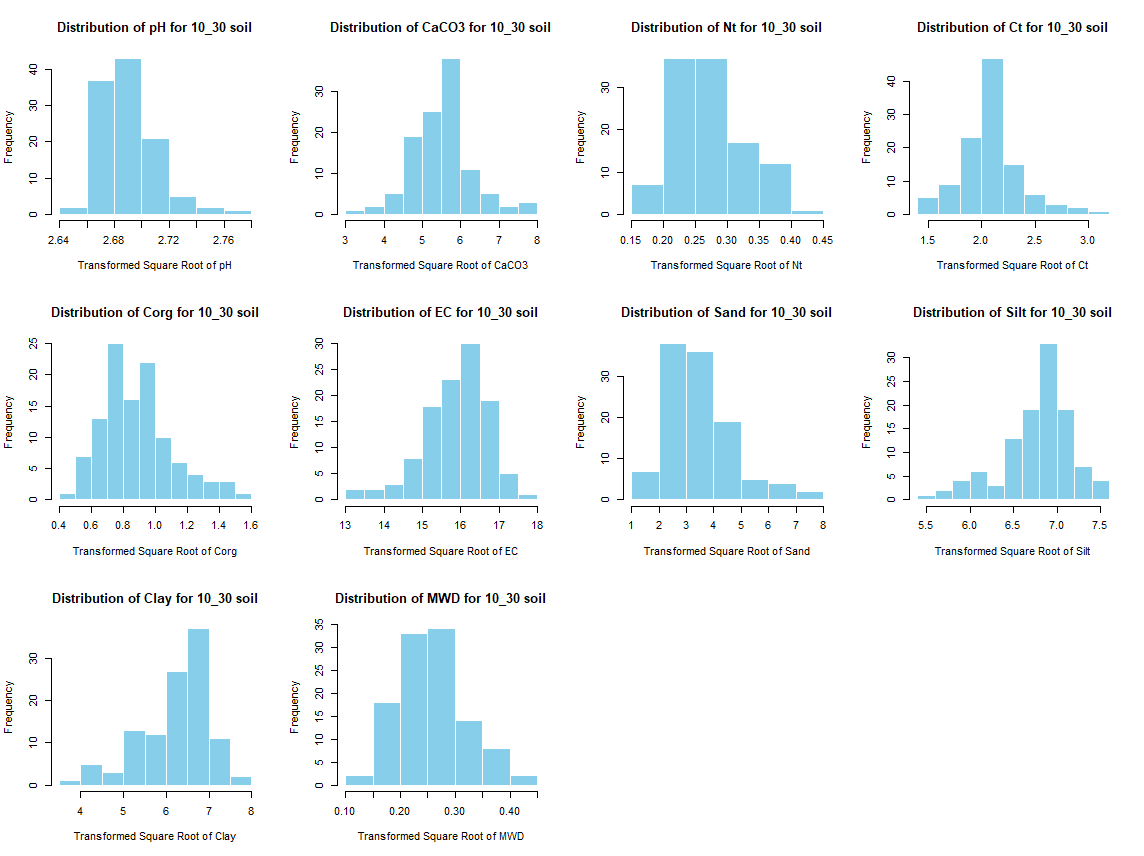
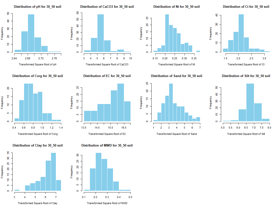
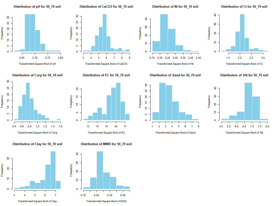
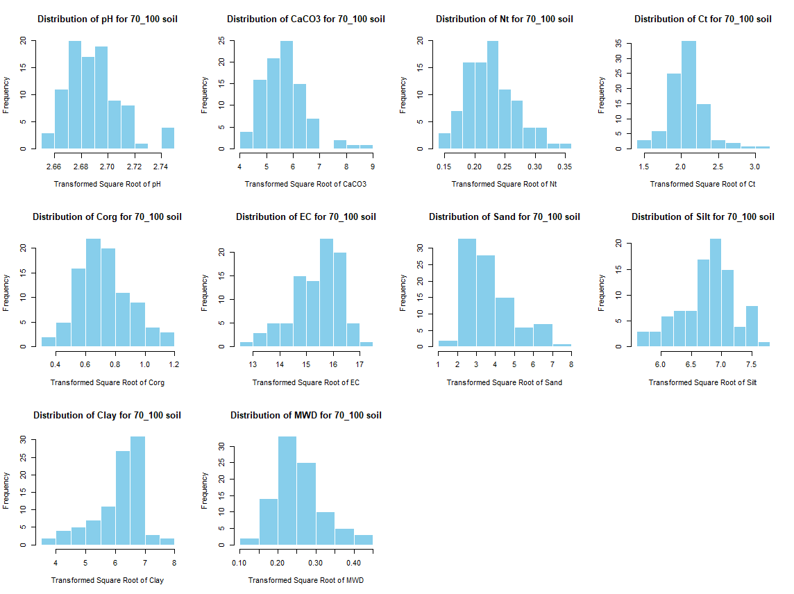
for (i in 1:length(soil_infos)) {
windows(width = 12, height = 9)
par(mfrow = c(3, 4))
for (j in 4:length(soil_infos[[1]])) {
hist(sqrt(soil_infos[[i]][, j]), main = paste0("Distribution of ", names(soil_infos[[i]][j]), " for ", names(soil_infos[i]) ," soil"),
xlab = paste0("Transformed Square Root of ", names(soil_infos[[i]][j])), col = "skyblue", border = "white")
}
savePlot(paste0("./export/preprocess/Histogram_sqrt_", names(soil_infos[i]), "_soil.png"), type = "png")
par(mfrow = c(1, 1))
dev.off()
windows(width = 12, height = 9)
par(mfrow = c(3, 4))
for (j in 4:length(soil_infos[[1]])) {
hist(soil_infos[[i]][, j], main = paste0("Distribution of ", names(soil_infos[[i]][j]), " for ", names(soil_infos[i]) ," soil"),
xlab = paste0("Distribution of ", names(soil_infos[[i]][j])), col = "skyblue", border = "white")
}
savePlot(paste0("./export/preprocess/Histogram_", names(soil_infos[i]), "_soil.png"), type = "png")
par(mfrow = c(1, 1))
dev.off()
}
dev.off() 
# 01.3 Set coordinates =========================================================

# Create a spatial dataframe and convert to WGS84 UTM 38 N coordinates

soil_infos_sp <- soil_infos

for (i in 1:length(soil_infos)) {
  soil_infos_sp[[i]] <- st_as_sf(soil_infos_sp[[i]], coords = c("Longitude", "Latitude"), crs = 4326)
  soil_infos_sp[[i]] <-st_transform(soil_infos_sp[[i]], crs = 32638)
}

mapview(soil_infos_sp[[1]]) + mapview(soil_infos_sp[[2]], col.regions = "red") + mapview(soil_infos_sp[[3]], col.regions = "green") +
  mapview(soil_infos_sp[[4]], col.regions = "pink") + mapview(soil_infos_sp[[5]], col.regions = "darkgrey")
7.2.3 Prepare the covariates
# 01.4 Import covariates raster ================================================
Landsat <- list.files("./data/Landsat/", full.names = TRUE)
Landsat <- Landsat[!grepl("raw", Landsat, ignore.case = TRUE)]
Landsat <- rast(Landsat)
Sentinel <- list.files("./data/Sentinel/", full.names = TRUE)
Sentinel <- Sentinel[!grepl("raw", Sentinel, ignore.case = TRUE)]
Sentinel <- rast(Sentinel)
Terrain <- list.files("./SAGA/", pattern = "*sg-grd-z" , full.names = TRUE)
Terrain <- rast(Terrain[-c(2,4,7,8,9,11,15,25)])
names(Terrain)[names(Terrain) == "DEM_raw [no sinks] [Smoothed]"] <- "DEM"
names(Terrain)[names(Terrain) == "Landforms"] <- "Surface Landform"
names(Terrain)[names(Terrain) == "LS Factor"] <- "Total Catchment Area"
names(Terrain)[names(Terrain) == "Vertical Distance to Channel Network"] <- "Channel Network Distance"
Terrain <- Terrain[[order(names(Terrain))]]
Sentinel <- list.files("./data/Sentinel/", full.names = TRUE)
Sentinel <- Sentinel[!grepl("raw", Sentinel, ignore.case = TRUE)]
Sentinel <- rast(Sentinel)
Others <- list.files("./data/Others/", full.names = TRUE)
Others <- Others[!grepl("raw", Others, ignore.case = TRUE)]
Others <- Others[!grepl("DEM", Others, ignore.case = TRUE)]
Others <- rast(Others)
Others_names <- list.files("./data/Others/")
Others_names <- Others_names[!grepl("raw", Others_names, ignore.case = TRUE)]
Others_names <- Others_names[!grepl("DEM", Others_names, ignore.case = TRUE)]
names(Others) <- gsub("\\.tif$", "", Others_names)
Modis <- list.files("./data/MODIS/", full.names = TRUE)
Modis <- Modis[!grepl("raw", Modis, ignore.case = TRUE)]
Modis <- rast(Modis)
names(Modis) <- gsub("\\_raw$", "", names(Modis))
# RS Landsat 8
Landsat$Landsat8_NDWI <- (Landsat$Landsat8_green_2021_MedianComposite - Landsat$Landsat8_NIR_2021_MedianComposite)/(Landsat$Landsat8_green_2021_MedianComposite + Landsat$Landsat8_NIR_2021_MedianComposite)
Landsat$Landsat8_NDVI <- (Landsat$Landsat8_NIR_2021_MedianComposite - Landsat$Landsat8_red_2021_MedianComposite)/(Landsat$Landsat8_NIR_2021_MedianComposite + Landsat$Landsat8_red_2021_MedianComposite)
Landsat$EVI <- 2.5 * ((Landsat$Landsat8_NIR_2021_MedianComposite - Landsat$Landsat8_red_2021_MedianComposite)/((Landsat$Landsat8_NIR_2021_MedianComposite + 6 * Landsat$Landsat8_red_2021_MedianComposite) - (7.5*Landsat$Landsat8_blue_2021_MedianComposite) + 1))
Landsat$SAVI <- 1.5 * ((Landsat$Landsat8_NIR_2021_MedianComposite - Landsat$Landsat8_red_2021_MedianComposite) / (Landsat$Landsat8_NIR_2021_MedianComposite + Landsat$Landsat8_red_2021_MedianComposite + 0.5)) #Enhanced Vegetation Index
Landsat$TVI <- sqrt(Landsat$Landsat8_NDVI + 0.5)
Landsat$NDMI <- (Landsat$Landsat8_NIR_2021_MedianComposite - Landsat$Landsat8_SWIR1_2021_MedianComposite)/(Landsat$Landsat8_NIR_2021_MedianComposite + Landsat$Landsat8_SWIR1_2021_MedianComposite) # normilized difference moisture index
Landsat$COSRI <- Landsat$Landsat8_NDVI * ((Landsat$Landsat8_blue_2021_MedianComposite + Landsat$Landsat8_green_2021_MedianComposite)/(Landsat$Landsat8_red_2021_MedianComposite + Landsat$Landsat8_NIR_2021_MedianComposite)) # Combined Specteral Response Index
Landsat$LSWI <- (Landsat$Landsat8_NIR_2021_MedianComposite - Landsat$Landsat8_SWIR1_2021_MedianComposite) / (Landsat$Landsat8_NIR_2021_MedianComposite + Landsat$Landsat8_SWIR1_2021_MedianComposite)
Landsat$BrightnessIndex <- sqrt((Landsat$Landsat8_red_2021_MedianComposite^2) + (Landsat$Landsat8_NIR_2021_MedianComposite^2))
Landsat$ClayIndex <- Landsat$Landsat8_SWIR1_2021_MedianComposite / Landsat$Landsat8_SWIR2_2021_MedianComposite
Landsat$SalinityIndex <- (Landsat$Landsat8_SWIR1_2021_MedianComposite - Landsat$Landsat8_SWIR2_2021_MedianComposite) / (Landsat$Landsat8_SWIR1_2021_MedianComposite - Landsat$Landsat8_NIR_2021_MedianComposite)
Landsat$CarbonateIndex <- Landsat$Landsat8_red_2021_MedianComposite / Landsat$Landsat8_green_2021_MedianComposite
Landsat$GypsumIndex <- (Landsat$Landsat8_SWIR1_2021_MedianComposite - Landsat$Landsat8_SWIR2_2021_MedianComposite) / (Landsat$Landsat8_SWIR1_2021_MedianComposite + Landsat$Landsat8_SWIR2_2021_MedianComposite)
# RS Sentinel 2
Sentinel$Sentinel2_NDWI <- (Sentinel$Sentinel2_green_2021_MedianComposite - Sentinel$Sentinel2_NIR_2021_MedianComposite) / (Sentinel$Sentinel2_green_2021_MedianComposite + Sentinel$Sentinel2_NIR_2021_MedianComposite)
Sentinel$Sentinel2_NDVI <- (Sentinel$Sentinel2_NIR_2021_MedianComposite - Sentinel$Sentinel2_red_2021_MedianComposite) / (Sentinel$Sentinel2_NIR_2021_MedianComposite + Sentinel$Sentinel2_red_2021_MedianComposite)
Sentinel$EVI <- 2.5 * ((Sentinel$Sentinel2_NIR_2021_MedianComposite - Sentinel$Sentinel2_red_2021_MedianComposite) / ((Sentinel$Sentinel2_NIR_2021_MedianComposite + 6 * Sentinel$Sentinel2_red_2021_MedianComposite) - (7.5 * Sentinel$Sentinel2_blue_2021_MedianComposite) + 1))
Sentinel$SAVI <- 1.5 * ((Sentinel$Sentinel2_NIR_2021_MedianComposite - Sentinel$Sentinel2_red_2021_MedianComposite) / (Sentinel$Sentinel2_NIR_2021_MedianComposite + Sentinel$Sentinel2_red_2021_MedianComposite + 0.5))
Sentinel$TVI <- sqrt(Sentinel$Sentinel2_NDVI + 0.5)
Sentinel$NDMI <- (Sentinel$Sentinel2_NIR_2021_MedianComposite - Sentinel$Sentinel2_SWIR1_2021_MedianComposite) / (Sentinel$Sentinel2_NIR_2021_MedianComposite + Sentinel$Sentinel2_SWIR1_2021_MedianComposite) # normilized difference moisture index
Sentinel$COSRI <- Sentinel$Sentinel2_NDVI * ((Sentinel$Sentinel2_blue_2021_MedianComposite + Sentinel$Sentinel2_green_2021_MedianComposite)/(Sentinel$Sentinel2_red_2021_MedianComposite + Sentinel$Sentinel2_NIR_2021_MedianComposite)) # Combined Specteral Response Index
Sentinel$LSWI <- (Sentinel$Sentinel2_NIR_2021_MedianComposite - Sentinel$Sentinel2_SWIR1_2021_MedianComposite) / (Sentinel$Sentinel2_NIR_2021_MedianComposite + Sentinel$Sentinel2_SWIR1_2021_MedianComposite)
Sentinel$BrightnessIndex <- sqrt((Sentinel$Sentinel2_red_2021_MedianComposite^2) + (Sentinel$Sentinel2_NIR_2021_MedianComposite^2))
Sentinel$ClayIndex <- Sentinel$Sentinel2_SWIR1_2021_MedianComposite / Sentinel$Sentinel2_SWIR2_2021_MedianComposite
Sentinel$SalinityIndex <- (Sentinel$Sentinel2_SWIR1_2021_MedianComposite - Sentinel$Sentinel2_SWIR2_2021_MedianComposite) / (Sentinel$Sentinel2_SWIR1_2021_MedianComposite - Sentinel$Sentinel2_NIR_2021_MedianComposite)
Sentinel$CarbonateIndex <- Sentinel$Sentinel2_red_2021_MedianComposite / Sentinel$Sentinel2_green_2021_MedianComposite
Sentinel$GypsumIndex <- (Sentinel$Sentinel2_SWIR1_2021_MedianComposite - Sentinel$Sentinel2_SWIR2_2021_MedianComposite) / (Sentinel$Sentinel2_SWIR1_2021_MedianComposite + Sentinel$Sentinel2_SWIR2_2021_MedianComposite)
# RS MODIS
Modis$SAVI <- 1.5 * ((Modis$MODIS_NIR - Modis$MODIS_Red) / (Modis$MODIS_NIR + Modis$MODIS_Red + 0.5))
Modis$TVI <- sqrt(Modis$MODIS_NDVI + 0.5)
Modis$BrightnessIndex <- sqrt((Modis$MODIS_Red^2) + (Modis$MODIS_NIR^2))
df_names <- data.frame()
for (i in 1:length(names(Terrain))) {
c <- paste0("TE.",i)
df_names[i,1] <- c
df_names[i,2] <- names(Terrain)[i]
}
t <- nrow(df_names)
for (i in 1:length(names(Landsat))) {
c <- paste0("LA.",i)
df_names[i+t,1] <- c
df_names[i+t,2] <- names(Landsat)[i]
}
t <- nrow(df_names)
for (i in 1:length(names(Sentinel))) {
c <- paste0("SE.",i)
df_names[i+t,1] <- c
df_names[i+t,2] <- names(Sentinel)[i]
}
t <- nrow(df_names)
for (i in 1:length(names(Modis))) {
c <- paste0("MO.",i)
df_names[i+t,1] <- c
df_names[i+t,2] <- names(Modis)[i]
}
t <- nrow(df_names)
for (i in 1:length(names(Others))) {
c <- paste0("OT.",i)
df_names[i+t,1] <- c
df_names[i+t,2] <- names(Others)[i]
}
write.table(df_names,"./data/Covariates_names_DSM.txt")
x <- c(Terrain, Landsat, Sentinel, Modis, Others)
names(x) <- df_names[,1]
writeRaster(x, "./data/Stack_layers_DSM.tif", overwrite = TRUE)
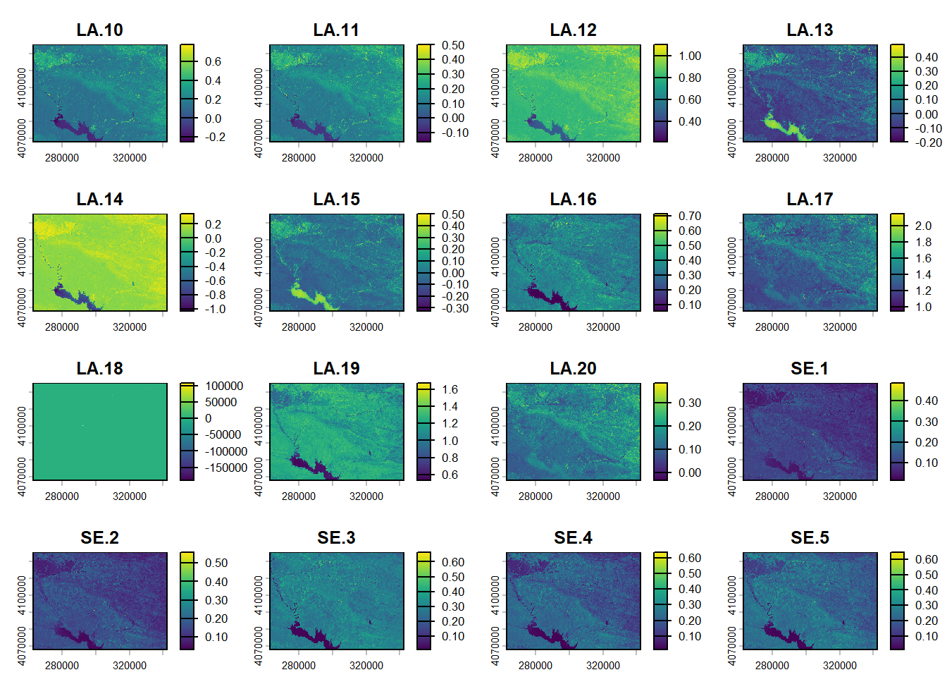
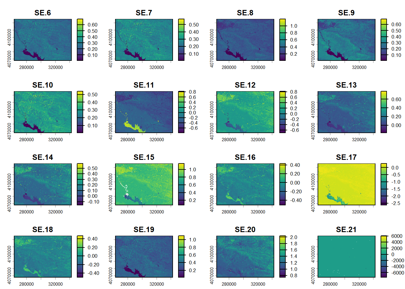
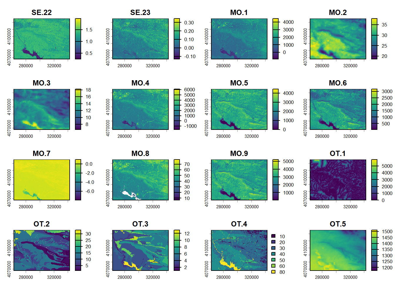
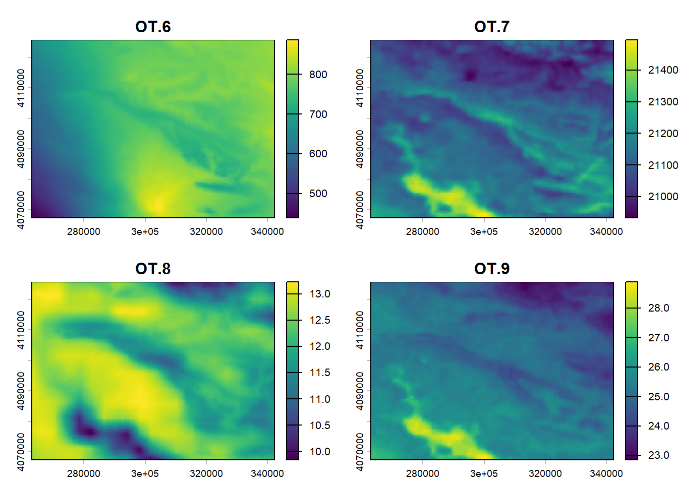
# 01.5 Plot the covariates maps ================================================
covariates <- rast("./data/Stack_layers_DSM.tif")
reduce <- aggregate(covariates, fact=10, fun=modal)
writeRaster(reduce, "./data/Stack_layers_DSM_reduce.tif", overwrite = TRUE)
plot(reduce)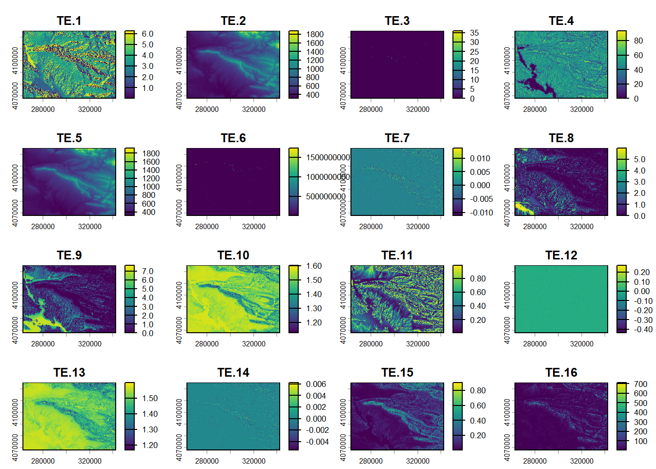
(#fig:script plot cov hide-1)Covariates from DSM.
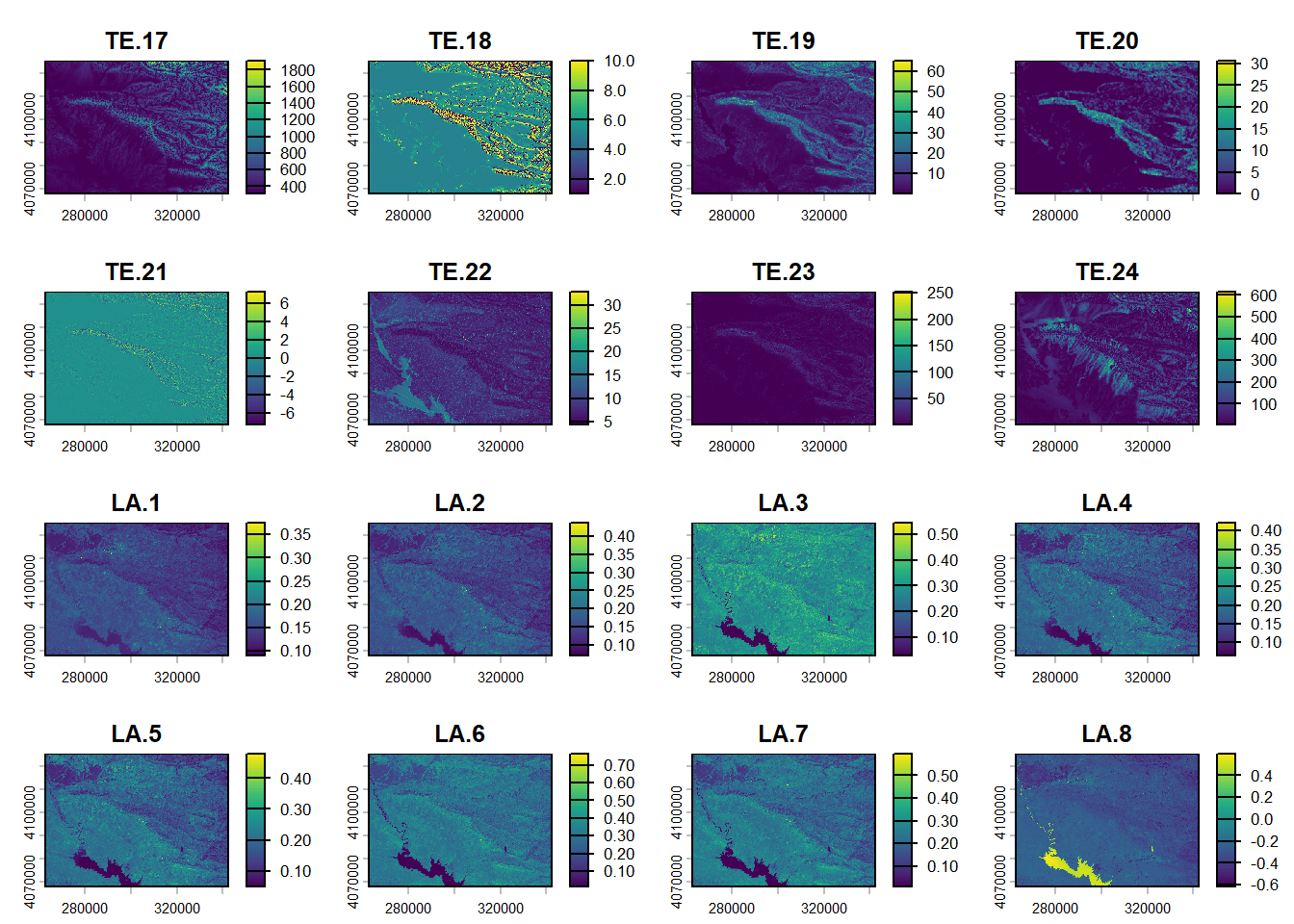
(#fig:script plot cov hide-2)Covariates from DSM.
(#fig:script plot cov hide-3)Covariates from DSM.
(#fig:script plot cov hide-4)Covariates from DSM.
(#fig:script plot cov hide-5)Covariates from DSM.
(#fig:script plot cov hide-6)Covariates from DSM.
# 01.6 Extract the values ======================================================

# Extract the values of each band for the sampling location

df_cov <- soil_infos_sp

for (i in 1:length(df_cov)) {
  df_cov[[i]] <- extract(covariates, df_cov[[i]], method='simple')
  df_cov[[i]] <- as.data.frame(df_cov[[i]])
  write.csv(df_cov[[i]], paste0("./data/df_",names(df_cov[i]),"_cov_DSM.csv"))
}

# 01.7 Export and save data ====================================================

save(df_cov, soil_infos_sp, file = "./export/save/Preprocess.RData")
rm(list = ls())


# 02 Check the data ############################################################

# 02.1 Import the data and merge ===============================================
make_subdir <- function(parent_dir, subdir_name) {
  path <- file.path(parent_dir, subdir_name)

  if (!dir.exists(path)) {
    dir.create(path, recursive = TRUE)
    message("✅  Folder created", path)
  } else {
    message("ℹ️ Existing folder : ", path)
  }

  return(path)
}

make_subdir("./export", "preprocess")


load(file = "./export/save/Preprocess.RData")

SoilCov <- df_cov
for (i in 1:length(SoilCov)) {
  ID <- 1:nrow(SoilCov[[i]])
  SoilCov[[i]] <- cbind(df_cov[[i]], ID, st_drop_geometry(soil_infos_sp[[i]]))
  cat("There is ", sum(is.na(SoilCov[[i]])== TRUE), "Na values in ", names(SoilCov[i])," soil list \n")
}


# 02.2 Plot and export the correlation matrix ==================================

for (i in 1:length(df_cov)) {
  pdf(paste0("./export/preprocess/Correlation_",names(df_cov[i]), ".pdf"),    # File name
      width = 40, height = 40,  # Width and height in inches
      bg = "white",          # Background color
      colormodel = "cmyk")   # Color model


  # Correlation of the data (remove discrete data)
  corrplot(cor(df_cov[[i]][,-c(1,79:81)]),  method = "color", col = viridis(200),
           type = "upper",
           addCoef.col = "black", # Add coefficient of correlation
           tl.col = "black", tl.srt = 45, # Text label color and rotation
           number.cex = 0.7, # Size of the text labels
           cl.cex = 0.7, # Size of the color legend text
           cl.lim = c(-1, 1)) # Color legend limits

  dev.off()

}
(#fig:script extract covariates hide-1)Auto-correlation plot 0_10

(#fig:script extract covariates hide-2)Auto-correlation plot 10_30

(#fig:script extract covariates hide-3)Auto-correlation plot 30_50

(#fig:script extract covariates hide-4)Auto-correlation plot 50_70
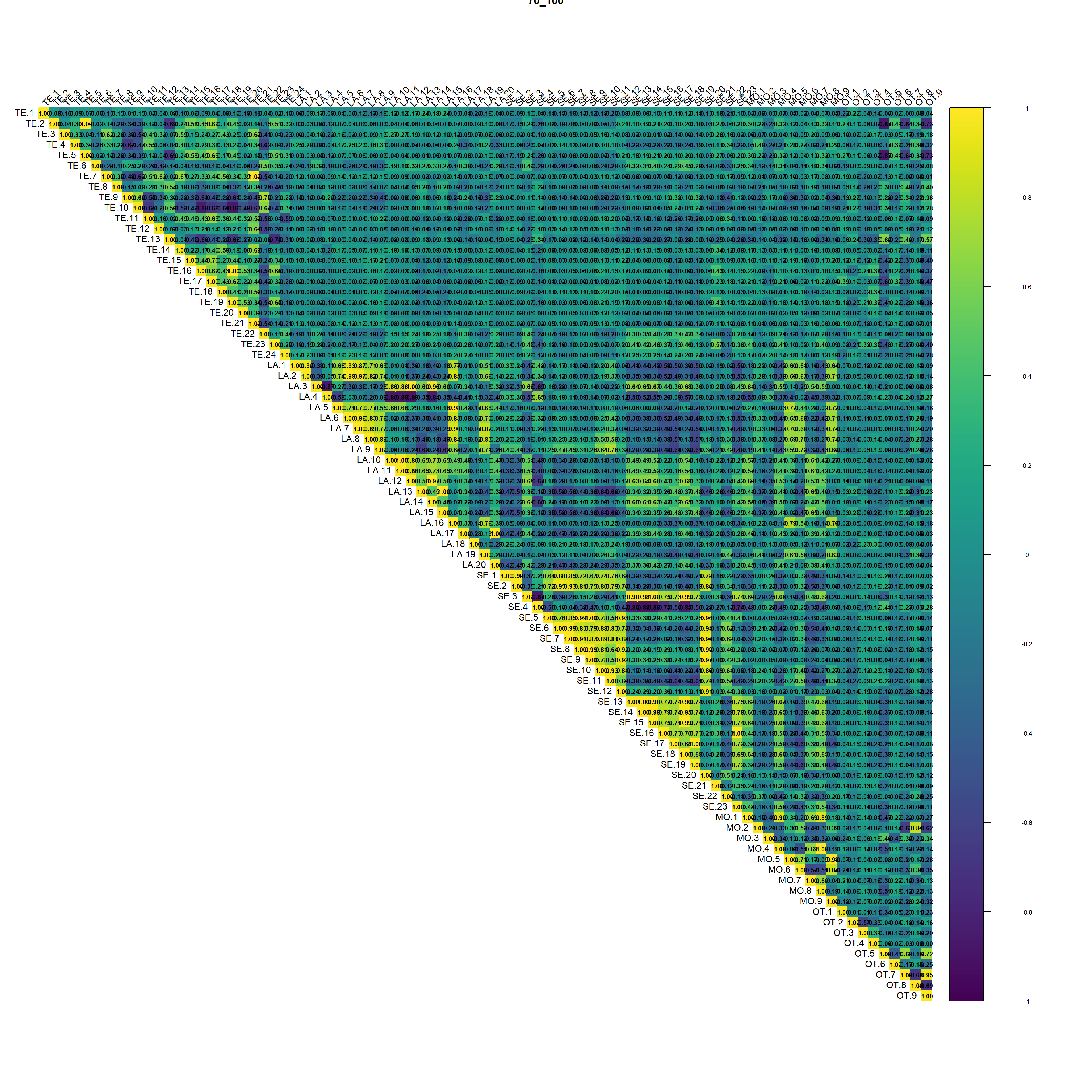
(#fig:script extract covariates hide-5)Auto-correlation plot 70_100
Regarding the correlation plot the Landsat and Sentinel bands are the ones with the higher correlation followed by terrain derivatives from DEM.
# 02.3 Select with VIF correlation =============================================

vif <- df_cov
vif_plot <- df_cov

for (i in 1:length(df_cov)) {
  vif[[i]] <-vifcor(df_cov[[i]], th=0.8)
  vif_df <- as.data.frame(vif[[i]]@results)
  write.table(vif_df, paste0("./export/VIF/vif_results_",names(df_cov[i]) ,"_soil.txt"))

  vif_plot[[i]] <- ggplot(vif_df, aes(x = reorder(Variables, VIF), y = VIF)) +
    geom_bar(stat = "identity", fill = "lightblue") +
    coord_flip() +
    theme_minimal() +
    labs(title = paste0("VIF Values for ", names(df_cov[i]) ," soil"), x = "Variables", y = "VIF") +
    theme(axis.text.x = element_text(angle = 45, hjust = 1))

  ggsave(paste0("./export/VIF/VIF_", names(df_cov[i]),"_soil.png"), vif_plot[[i]], width = 12, height = 8)
  ggsave(paste0("./export/VIF/VIF_", names(df_cov[i]),"_soil.pdf"), vif_plot[[i]], width = 12, height = 8)
}

# 02.4 Statistics ==============================================================
increments <- c("0_10", "10_30", "30_50", "50_70", "70_100")

make_subdir("./export", "Boruta")

for (depth in increments) {
  make_subdir("./export/Boruta", depth)
  make_subdir("./export/RFE", depth)
  make_subdir("./export/preprocess", depth)
# Basic statistics
  print(names(SoilCov[[depth]]))
  print(nrow(SoilCov[[depth]]))
# If necessary
  SoilCov[[depth]] <- na.omit(SoilCov[[depth]])
  print(head(SoilCov[[depth]]))
  sapply(SoilCov[[depth]], class)
  print(summary(SoilCov[[depth]]))
}
7.2.4 ALR transformation
# 03 Check covariates influences ###############################################
Cov <- list()
nzv_vars <- list()
cl <- makeCluster(6)
registerDoParallel(cl)
# 03.1 Transform the soiltexture and remove nzv ================================
for (depth in increments) {
depth_name <- gsub("_", " - ", depth)
SoilCovMLCon <- SoilCov[[depth]][,-c(1,87:88)] # Remove ID and site name
NumCovLayer = 85 # define number of covariate layer after hot coding
StartTargetCov = NumCovLayer + 1 # start column after all covariates
NumDataCol= ncol(SoilCovMLCon) # number of column in all data set
# Remove and save NZV
nzv <- nearZeroVar(SoilCovMLCon[,1:NumCovLayer], saveMetrics = TRUE)
nzv_vars[[depth]] <- rownames(nzv)[nzv$nzv == TRUE]
print(rownames(nzv)[nzv$nzv == TRUE])
# Realise the PSF transformation
texture_df <- SoilCovMLCon[,c((NumDataCol-3):(NumDataCol-1))]
colnames(texture_df) <- c("SAND","SILT", "CLAY")
texture_df <- TT.normalise.sum(texture_df, css.names = c("SAND","SILT", "CLAY"))
colnames(texture_df) <- colnames(SoilCovMLCon[,c((NumDataCol-3):(NumDataCol-1))])
alr_df <- as.data.frame(alr(texture_df)) # Additive-log ratio with Sand/Clay and Silt/Clay (last column is taken)
colnames(alr_df) <- c("alr.Sand", "alr.Silt")
SoilCovMLCon <- SoilCovMLCon[,-c((NumDataCol-3):(NumDataCol-1))]
SoilCovMLCon <- cbind(SoilCovMLCon, alr_df, texture_df)
NumDataCol <- (NumDataCol -1)
Cov[[depth]] <- SoilCovMLCon
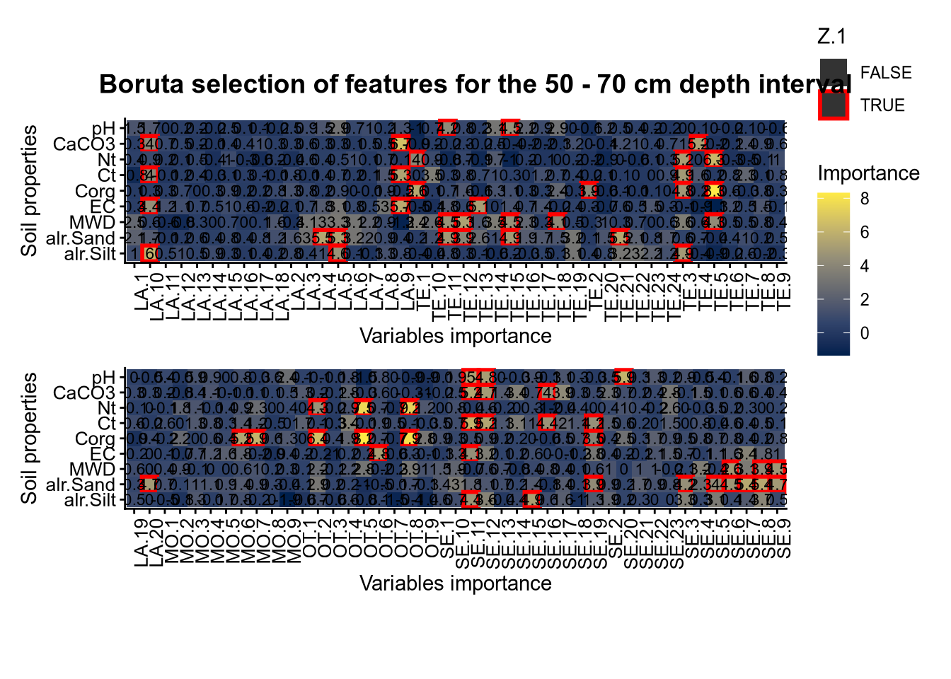
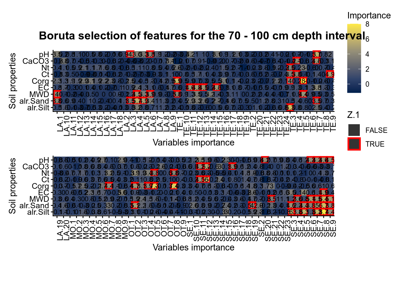
}7.2.5 Boruta and RFE selections
# 03.3 Boruta selection =========================================================
FormulaMLCon <- list()
Preprocess <- list()
for (i in 1:(ncol(Cov[[1]]) - NumCovLayer - 3)) {
FormulaMLCon[[i]] = as.formula(paste(names(Cov[[1]])[NumCovLayer+i]," ~ ",paste(names(Cov[[1]])[1:NumCovLayer],collapse="+")))
}
# Define traincontrol
TrainControl <- trainControl(method="repeatedcv", 10, 3, allowParallel = TRUE, savePredictions=TRUE)
TrainControlRF <- rfeControl(functions = rfFuncs, method = "repeatedcv", 10, 3, allowParallel = TRUE)
seed=1070
for (depth in increments) {
depth_name <- gsub("_", " - ", depth)
Boruta = list()
BorutaLabels = list()
Boruta_covariates = list()
SoilCovMLCon <- Cov[[depth]]
cli_progress_bar(
format = "Boruta {.val {depth}} {.val {var}} {cli::pb_bar} {cli::pb_percent} [{cli::pb_current}/{cli::pb_total}] | \ ETA: {cli::pb_eta} - Time elapsed: {cli::pb_elapsed_clock}",
total = length(FormulaMLCon),
clear = FALSE)
# Individual plots
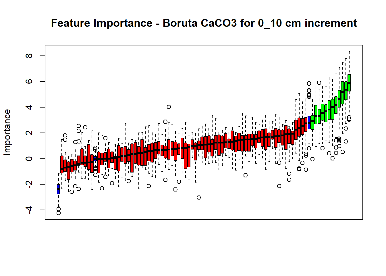
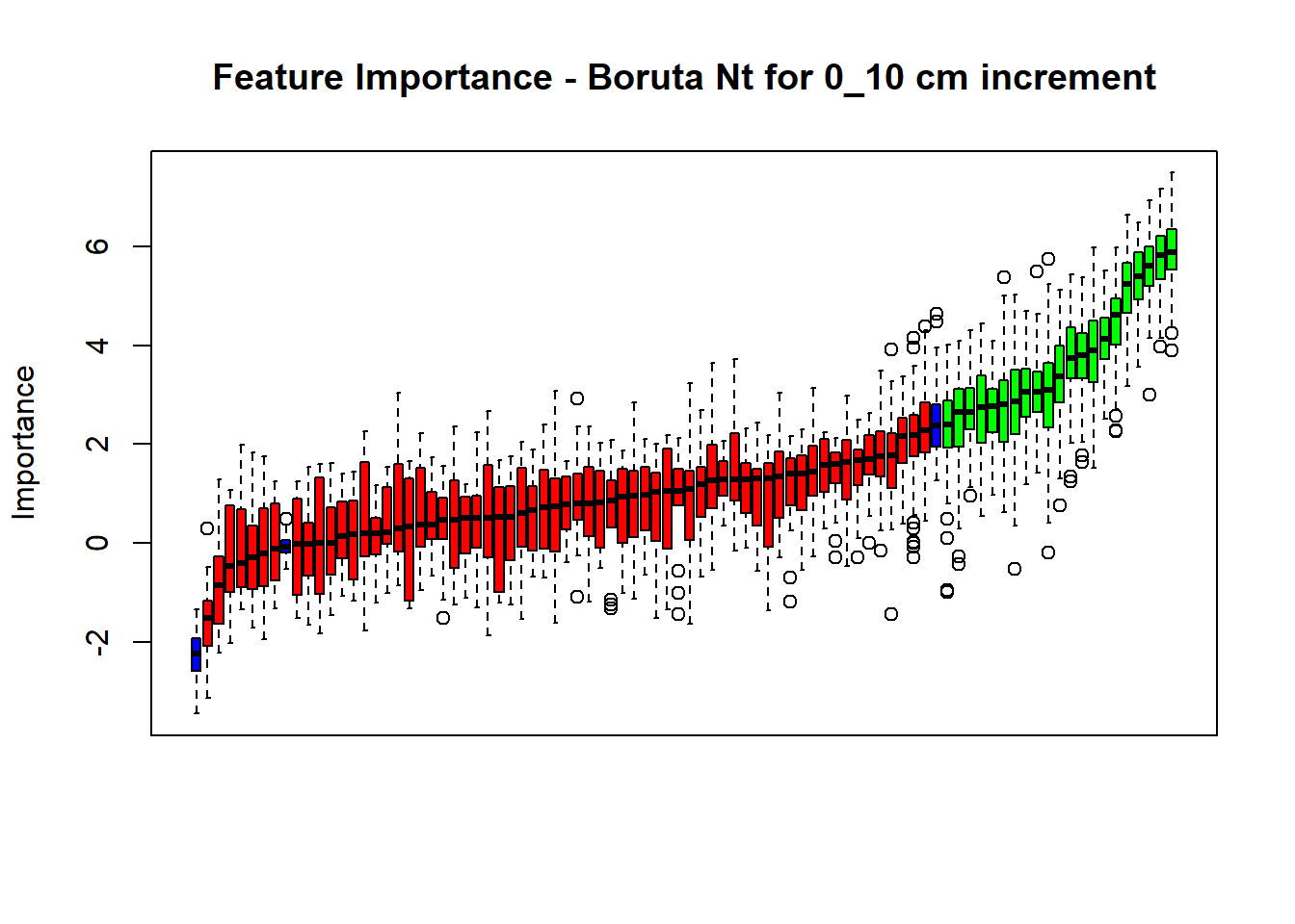
for (i in 1:length(FormulaMLCon)) {
var <- names(SoilCovMLCon)[NumCovLayer+i]
set.seed(seed)
Boruta[[i]] <- Boruta(FormulaMLCon[[i]], data = SoilCovMLCon, rfeControl = TrainControl)
BorutaBank <- TentativeRoughFix(Boruta[[i]])
pdf(paste0("./export/boruta/", depth,"/Boruta_",names(SoilCovMLCon)[NumCovLayer+i], "_for_",depth,"_soil.pdf"), # File name
width = 8, height = 8, # Width and height in inches
bg = "white", # Background color
colormodel = "cmyk") # Color model
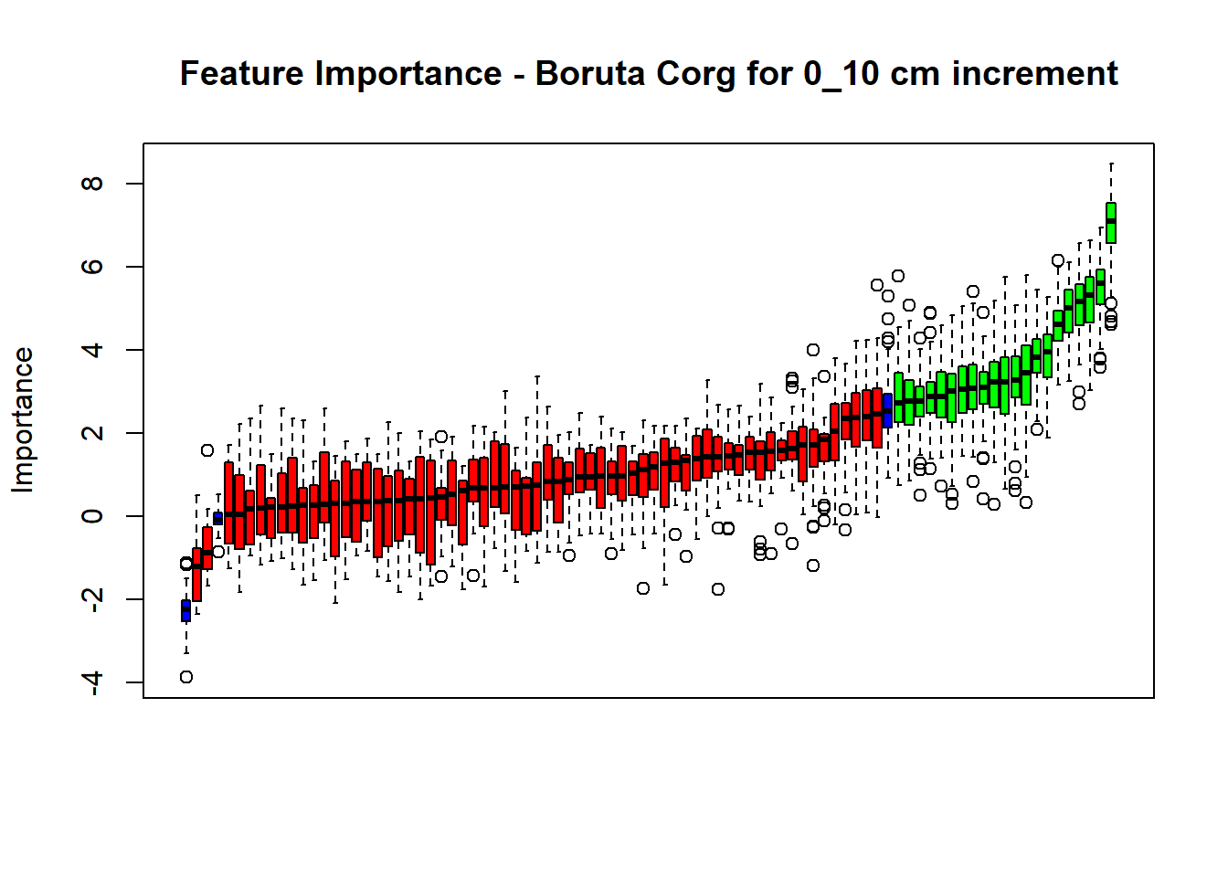
plot(BorutaBank, xlab = "", xaxt = "n",
main=paste0("Feature Importance - Boruta ",names(SoilCovMLCon)[NumCovLayer+i]," for ", depth_name ," cm increment"))
lz <- lapply(1:ncol(BorutaBank$ImpHistory),
function(j)BorutaBank$ImpHistory[is.finite(BorutaBank$ImpHistory[,j]),j])
names(lz) <- c(names(SoilCovMLCon)[1:NumCovLayer],c("sh_Max","sh_Mean","sh_Min"))
Labels <- sort(sapply(lz,median))
axis(side = 1,las=2,labels = names(Labels),at = 1:ncol(BorutaBank$ImpHistory),
cex.axis = 1)
dev.off() # Close the device
BorutaLabels[[i]] <- sapply(lz,median)
confirmed_features <- getSelectedAttributes(BorutaBank, withTentative = FALSE)
Boruta_covariates[[i]] <- cbind(SoilCovMLCon[, confirmed_features], SoilCovMLCon[, NumCovLayer + i])
colnames(Boruta_covariates[[i]]) <- c(confirmed_features,names(SoilCovMLCon)[NumCovLayer+i])
write.csv(data.frame(Boruta_covariates[[i]]), paste0("./export/boruta/", depth,"/Boruta_results_",names(SoilCovMLCon)[NumCovLayer+i], "_for_",depth,"_soil.csv"))
cli_progress_update()
}
cli_progress_done()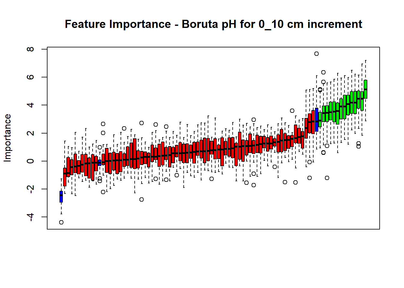
(#fig:Boruta hide-1)Boruta plot 0_10
(#fig:Boruta hide-2)Boruta plot 10_30
(#fig:Boruta hide-3)Boruta plot 30_50

(#fig:Boruta hide-4)Boruta plot 50_70
(#fig:Boruta hide-5)Boruta plot 70_100
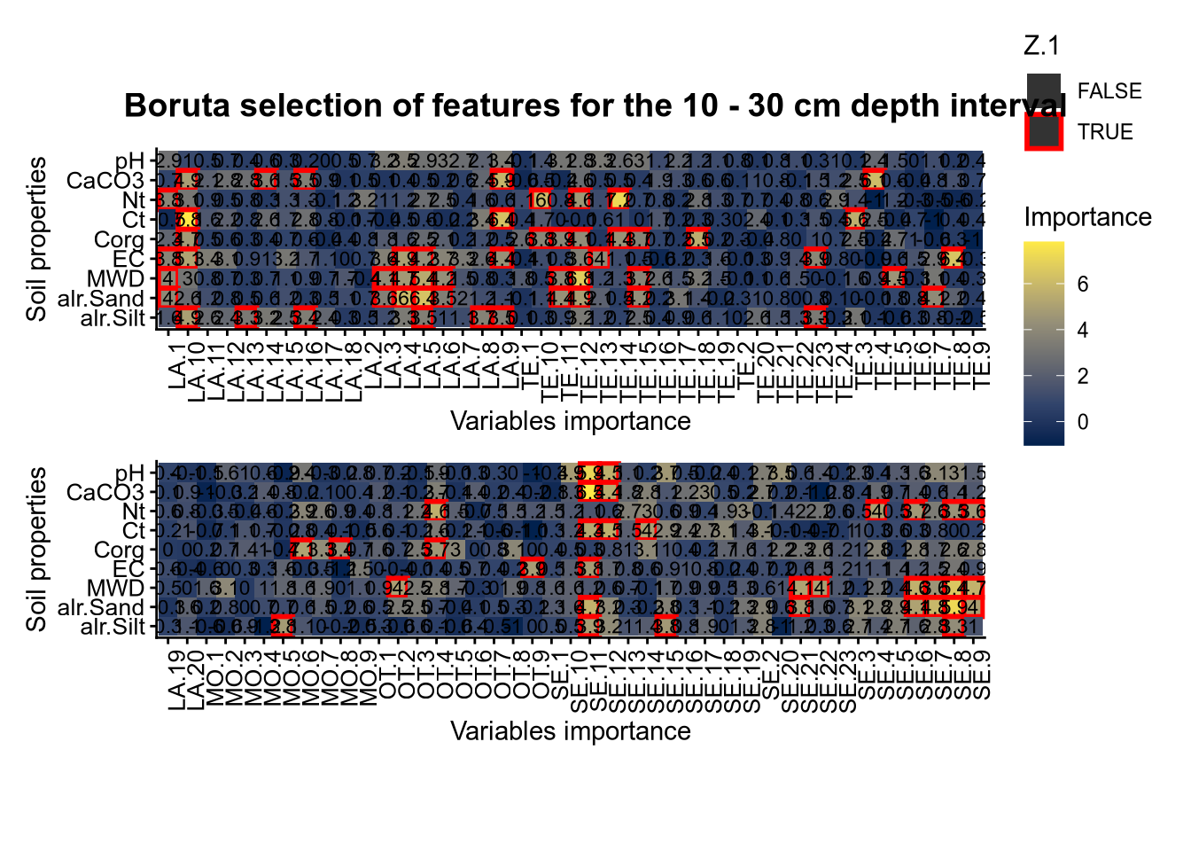
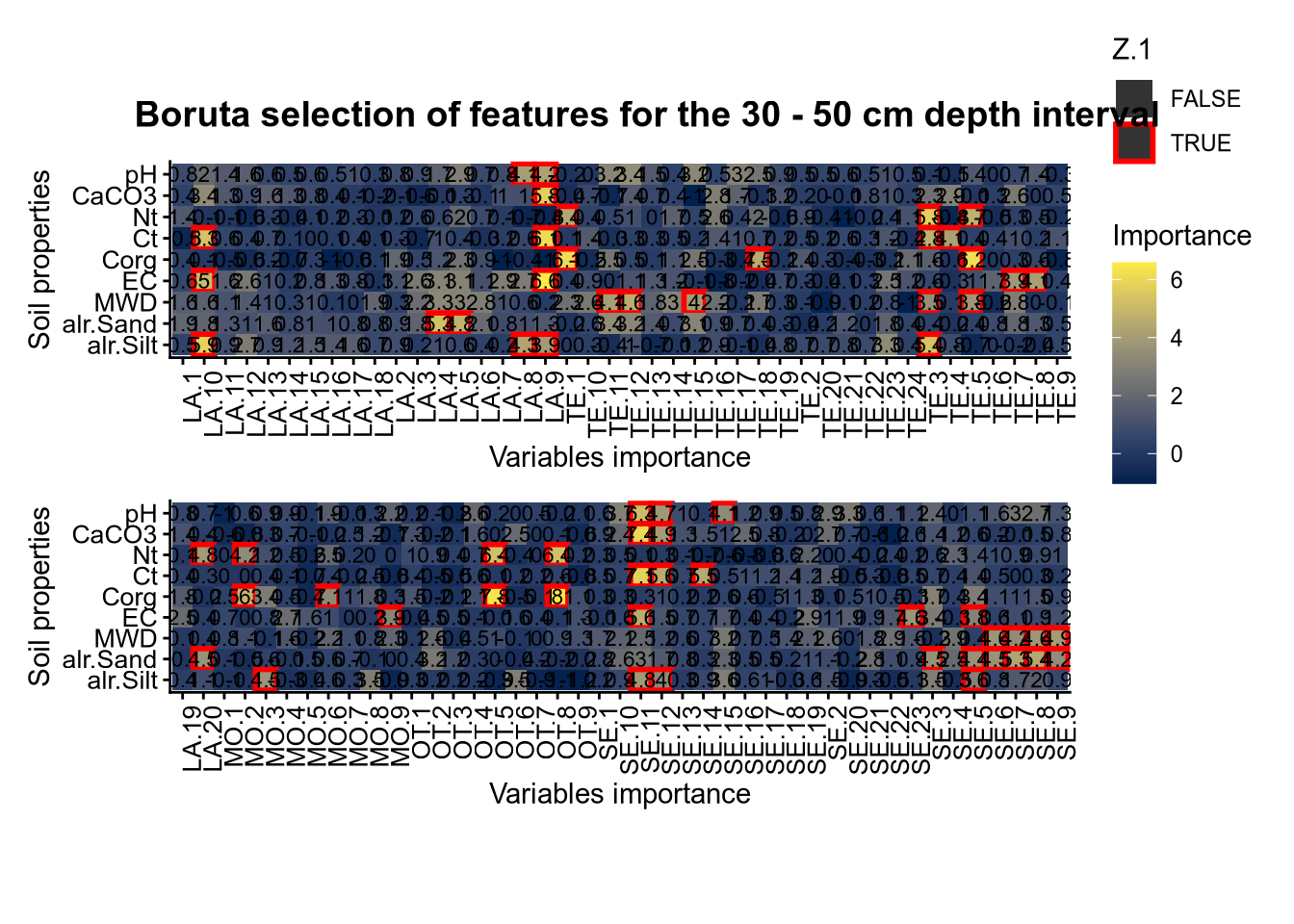
  # Combinned plot
  BorutaResultCon = data.frame();BorutaResultCon = data.frame(BorutaLabels[[1]])
  for (i in 2:length(FormulaMLCon)) {
    BorutaResultCon[i] = data.frame(BorutaLabels[[i]])}
  BorutaResultCon    = BorutaResultCon[c(1:NumCovLayer),]
  names(BorutaResultCon) <- names(SoilCovMLCon)[c(StartTargetCov:NumDataCol)]

  BorutaResultConT = data.frame();BorutaResultConT = data.frame(Boruta[[1]]$finalDecision == "Confirmed")
  for (i in 2:length(FormulaMLCon)) {
    BorutaResultConT[i] = data.frame(Boruta[[i]]$finalDecision == "Confirmed")}
  names(BorutaResultConT) <- names(SoilCovMLCon)[c(StartTargetCov:NumDataCol)]

  BorutaCovPlot = gather(BorutaResultCon,key,value);BorutaCovPlotT = gather(BorutaResultConT,key,value)
  BorutaCovPlot$cov = rep(row.names(BorutaResultCon), (NumDataCol-NumCovLayer))
  names(BorutaCovPlot) = c("Y","Z","X");BorutaCovPlot$Z.1 = BorutaCovPlotT$value
  BorutaCovPlot$Y = factor(BorutaCovPlot$Y);BorutaCovPlot$X = factor(BorutaCovPlot$X)
  BorutaCovPlot$Z.1 <- as.logical(BorutaCovPlot$Z.1)
  BorutaCovPlot$Y = factor(BorutaCovPlot$Y, levels = rev(unique(BorutaCovPlot$Y)))

  # Split into two groups
  df1 <- BorutaCovPlot[BorutaCovPlot$X %in% unique(BorutaCovPlot$X)[1:42], ]
  df2 <- BorutaCovPlot[BorutaCovPlot$X %in% unique(BorutaCovPlot$X)[(43):length(unique(BorutaCovPlot$X))], ]

  # First part
  p1 <- ggplot(df1, aes(x = X, y = Y)) +
    geom_tile(aes(fill = Z, colour = Z.1), size = 1) +
    labs(x = "Variables importance", y = "Soil properties", fill = "Importance") +
    theme_classic() +
    scale_fill_viridis_c(option = "E") +
    scale_color_manual(values = c('#00000000', 'red')) +
    theme(axis.text.x = element_text(colour = "black", size = 10, angle = 90, hjust = 1),
          axis.text.y = element_text(colour = "black", size = 10),
          legend.position = "right") +
    geom_text(aes(label = round(Z, 1)), cex = 3) +
    coord_flip() +
    coord_equal()

  # Second part
  p2 <- ggplot(df2, aes(x = X, y = Y)) +
    geom_tile(aes(fill = Z, colour = Z.1), size = 1, show.legend = FALSE) +
    labs(x = "Variables importance", y = "Soil properties", fill = "Importance") +
    theme_classic() +
    scale_fill_viridis_c(option = "E") +
    scale_color_manual(values = c('#00000000', 'red')) +
    theme(axis.text.x = element_text(colour = "black", size = 10, angle = 90, hjust = 1),
          axis.text.y = element_text(colour = "black", size = 10)) +
    geom_text(aes(label = round(Z, 1)), cex = 3) +
    coord_flip() +
    coord_equal()

  # Combinne poth plot
  FigCovImpoBr <- (p1 / p2)  +
    plot_annotation(title = paste0("Boruta selection of features for the ", depth_name, " cm depth interval"),
                    theme = theme(plot.title = element_text(size = 14, face = "bold", hjust = 0.5)))

  ggsave(paste0("./export/boruta/", depth,"/Boruta_final_combinned_plot_", depth,"_soil.png"), FigCovImpoBr, width = 15, height = 8.5)
  ggsave(paste0("./export/boruta/", depth,"/Boruta_final_combinned_plot_", depth,"_soil.pdf"), FigCovImpoBr, width = 15, height = 8.5)
plot(FigCovImpoBr) 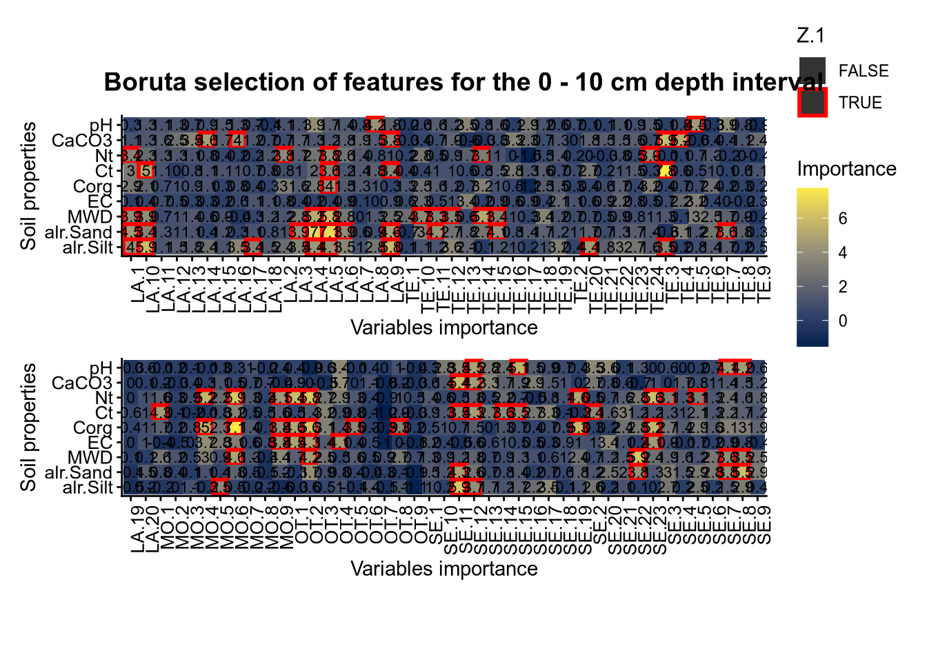
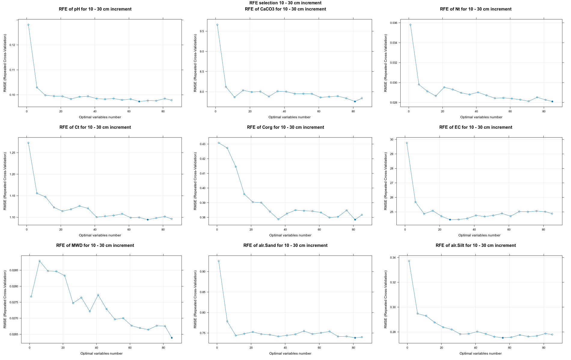
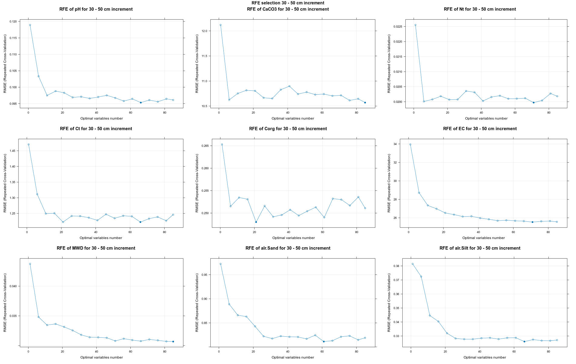
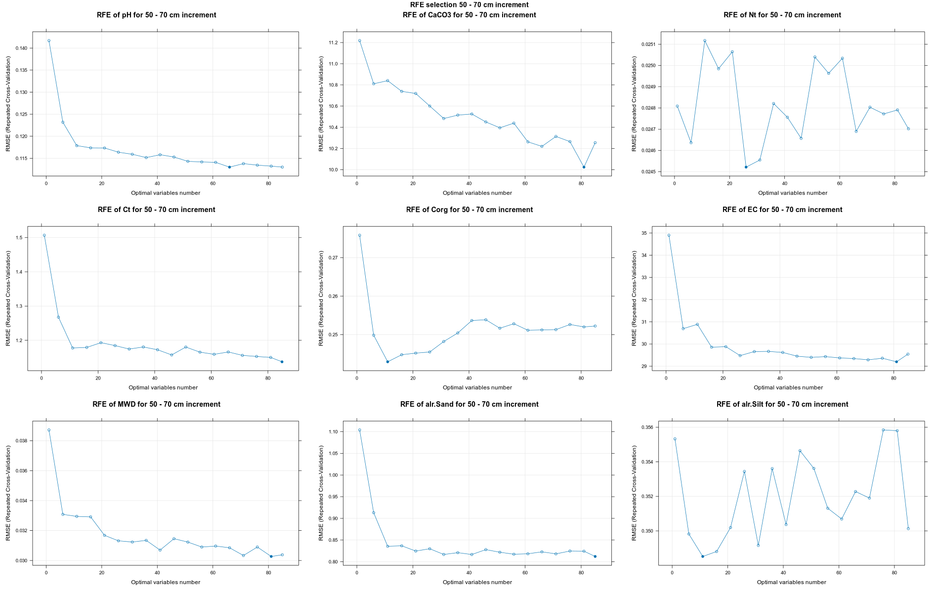
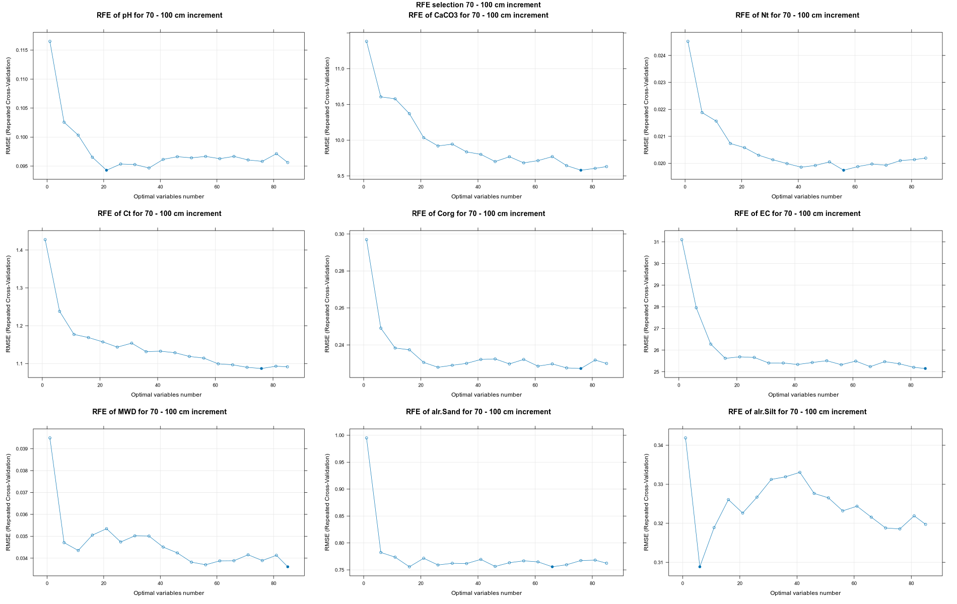
# 03.4 RFE covariate influence =================================================

  cli_progress_bar(
    format = "RFE {.val {depth}} {.val {var}} {cli::pb_bar} {cli::pb_percent} [{cli::pb_current}/{cli::pb_total}] | \ ETA: {cli::pb_eta} - Time elapsed: {cli::pb_elapsed_clock}",
    total = length(FormulaMLCon),
    clear = FALSE)

  ResultRFECon <- list()
  subsets= c(seq(1,NumCovLayer,5))

  for (i in 1:length(FormulaMLCon)) {
    var <- names(SoilCovMLCon)[NumCovLayer+i]
    set.seed(seed)
    ResultRFECon[[i]] <- rfe(FormulaMLCon[[i]], data=SoilCovMLCon,
                             sizes = subsets, rfeControl = TrainControlRF)
    cli_progress_update()
  }
  cli_progress_done()

  RFE_covariates <- list()
  for (i in 1:length(ResultRFECon)) {
    RFEpredictors <- predictors(ResultRFECon[[i]])
    RFE_covariates[[i]] <- cbind(SoilCovMLCon[, RFEpredictors], SoilCovMLCon[, NumCovLayer + i])
    colnames(RFE_covariates[[i]]) <- c(RFEpredictors, colnames(SoilCovMLCon[NumCovLayer+i]))
    write.table(data.frame(RFEpredictors), paste0("./export/RFE/", depth,"/RFE_results_",names(SoilCovMLCon)[NumCovLayer+i], "_for_",depth,"_soil.txt"))

  }

  PlotResultRFE =list()
  for (i in 1:length(ResultRFECon)) {
    trellis.par.set(caretTheme())

    PlotResultRFE[[i]] <- plot(ResultRFECon[[i]],
                              type = c("g", "o"),
                              main=paste0("RFE of ",names(SoilCovMLCon)[NumCovLayer+i]," for ",depth_name, " cm increment"),
                              xlab="Optimal variables number")

    pdf(paste0("./export/RFE/", depth,"/RFE_",names(SoilCovMLCon)[NumCovLayer+i], "_for_",depth,"_soil.pdf"),    # File name
        width = 12, height = 12,  # Width and height in inches
        bg = "white",          # Background color
        colormodel = "cmyk")   # Color model

    plot(PlotResultRFE[[i]])
    dev.off()
  }
# 03.5 Export results ==========================================================

  Preprocess[[depth]] <- list(
    NZV = nzv_vars,
    Cov = Cov,
    Selected_cov_boruta = Boruta_covariates,
    Boruta_full_fig = FigCovImpoBr,
    Boruta = Boruta,
    Selected_cov_RFE = RFE_covariates,
    RFE_fig = PlotResultRFE,
    RFE = ResultRFECon
  )
}

save(Preprocess, file = paste0("./export/save/Preprocess.RData"))

# 03.6 Covariates selection table ==============================================

cov_names <- read.table("./data/Covariates_names_DSM.txt")

conv <- data.frame(source = cov_names[,1],
  target  = paste(cov_names[,1], cov_names[,2], sep = "_"),
  stringsAsFactors = FALSE)

conversion <- setNames(conv$target, conv$source)
cov_list <- list()

# For Boruta
for (i in 1:length(Preprocess[[1]]$Selected_cov_boruta)) {
  cov <- list()
  for (depth in increments) {
    cov[[depth]] <- colnames(Preprocess[[depth]]$Selected_cov_boruta[[i]][1:length(Preprocess[[depth]]$Selected_cov_boruta[[i]])-1])
  }
  cov_combinned <- do.call(c, cov)
  cov_table <- conversion[cov_combinned]
  cov_table <- table(cov_table)

  df_top5 <- as.data.frame(
    head(sort(cov_table, decreasing = TRUE), 5)
  )

  colnames(df_top5) <- c("value", "occurrence")
  cov_list[[i]] <- data.frame(variable = colnames(Preprocess[[depth]]$Selected_cov_boruta[[i]][length(Preprocess[[depth]]$Selected_cov_boruta[[i]])]),
                       num.cov = c(paste0(length(Preprocess[["0_10"]]$Selected_cov_boruta[[i]])-1, "; ", length(Preprocess[["10_30"]]$Selected_cov_boruta[[i]])-1, "; ",
                                          length(Preprocess[["30_50"]]$Selected_cov_boruta[[i]])-1, "; ", length(Preprocess[["50_70"]]$Selected_cov_boruta[[i]])-1, "; ",
                                          length(Preprocess[["70_100"]]$Selected_cov_boruta[[i]])-1)),
                       top.cov = c(paste0(df_top5[1,1], "; ", df_top5[2,1], "; ", df_top5[3,1], "; ", df_top5[4,1], "; ", df_top5[5,1], "; "))
                       )
}

cov_combinned <- do.call(rbind, cov_list)
write.table(cov_combinned, "./export/boruta/Factors_selection.txt")

# For RFE
for (i in 1:length(Preprocess[[1]]$Selected_cov_RFE)) {
  cov <- list()
  for (depth in increments) {
    cov[[depth]] <- colnames(Preprocess[[depth]]$Selected_cov_RFE[[i]][1:length(Preprocess[[depth]]$Selected_cov_RFE[[i]])-1])
  }
  cov_combinned <- do.call(c, cov)
  cov_table <- conversion[cov_combinned]
  cov_table <- table(cov_table)

  df_top5 <- as.data.frame(
    head(sort(cov_table, decreasing = TRUE), 5)
  )

  colnames(df_top5) <- c("value", "occurrence")
  cov_list[[i]] <- data.frame(variable = colnames(Preprocess[[depth]]$Selected_cov_RFE[[i]][length(Preprocess[[depth]]$Selected_cov_RFE[[i]])]),
                              num.cov = c(paste0(length(Preprocess[["0_10"]]$Selected_cov_RFE[[i]])-1, "; ", length(Preprocess[["10_30"]]$Selected_cov_RFE[[i]])-1, "; ",
                                                 length(Preprocess[["30_50"]]$Selected_cov_RFE[[i]])-1, "; ", length(Preprocess[["50_70"]]$Selected_cov_RFE[[i]])-1, "; ",
                                                 length(Preprocess[["70_100"]]$Selected_cov_RFE[[i]])-1)),
                              top.cov = c(paste0(df_top5[1,1], "; ", df_top5[2,1], "; ", df_top5[3,1], "; ", df_top5[4,1], "; ", df_top5[5,1], "; "))
  )
}

cov_combinned <- do.call(rbind, cov_list)
write.table(cov_combinned, "./export/RFE/Factors_selection.txt")
7.3 Models developpement
7.3.1 Preparation of the environment
# 0 Environment setup ##########################################################

# 0.1 Prepare environment ======================================================

# Folder check
getwd()

# Set folder direction
setwd()

# Clean up workspace
rm(list = ls(all.names = TRUE))

# 0.2 Install packages =========================================================

install.packages("pacman")
#Install and load the "pacman" package (allow easier download of packages)
library(pacman)
pacman::p_load(ggplot2, caret, patchwork, quantregForest, readr, grid, gridExtra,
               dplyr, reshape2, cli, doParallel, compositions)

# 0.3 Show session infos =======================================================
R version 4.5.1 (2025-06-13 ucrt)
Platform: x86_64-w64-mingw32/x64
Running under: Windows 11 x64 (build 26200)
Matrix products: default
LAPACK version 3.12.1
locale:
[1] LC_COLLATE=French_France.utf8 LC_CTYPE=French_France.utf8 LC_MONETARY=French_France.utf8 LC_NUMERIC=C
[5] LC_TIME=French_France.utf8
time zone: Europe/Paris
tzcode source: internal
attached base packages:
[1] grid parallel stats graphics grDevices utils datasets methods base
other attached packages:
[1] compositions_2.0-9 doParallel_1.0.17 iterators_1.0.14 foreach_1.5.2 cli_3.6.5 reshape2_1.4.5
[7] dplyr_1.1.4 gridExtra_2.3 readr_2.1.6 quantregForest_1.3-7.1 RColorBrewer_1.1-3 randomForest_4.7-1.2
[13] patchwork_1.3.2 caret_7.0-1 lattice_0.22-7 ggplot2_4.0.1
loaded via a namespace (and not attached):
[1] DBI_1.2.3 pROC_1.19.0.1 tcltk_4.5.1 rlang_1.1.7 magrittr_2.0.4 otel_0.2.0
[7] e1071_1.7-17 compiler_4.5.1 png_0.1-8 vctrs_0.7.0 stringr_1.6.0 pkgconfig_2.0.3
[13] fastmap_1.2.0 leafem_0.2.5 rmarkdown_2.30 tzdb_0.5.0 prodlim_2025.04.28 purrr_1.2.1
[19] xfun_0.56 satellite_1.0.6 recipes_1.3.1 terra_1.8-93 R6_2.6.1 stringi_1.8.7
[25] parallelly_1.46.1 rpart_4.1.24 lubridate_1.9.4 Rcpp_1.1.1 bookdown_0.46 knitr_1.51
[31] future.apply_1.20.1 base64enc_0.1-3 pacman_0.5.1 Matrix_1.7-4 splines_4.5.1 nnet_7.3-20
[37] timechange_0.3.0 tidyselect_1.2.1 rstudioapi_0.18.0 dichromat_2.0-0.1 yaml_2.3.12 timeDate_4051.111
[43] codetools_0.2-20 listenv_0.10.0 tibble_3.3.1 plyr_1.8.9 withr_3.0.2 S7_0.2.1
[49] evaluate_1.0.5 future_1.69.0 survival_3.8-6 sf_1.0-24 bayesm_3.1-7 units_1.0-0
[55] proxy_0.4-29 pillar_1.11.1 tensorA_0.36.2.1 rsconnect_1.7.0 KernSmooth_2.23-26 stats4_4.5.1
[61] generics_0.1.4 sp_2.2-0 hms_1.1.4 scales_1.4.0 globals_0.18.0 class_7.3-23
[67] glue_1.8.0 tools_4.5.1 robustbase_0.99-6 data.table_1.18.0 ModelMetrics_1.2.2.2 gower_1.0.2
[73] crosstalk_1.2.2 ipred_0.9-15 nlme_3.1-168 raster_3.6-32 lava_1.8.2 DEoptimR_1.1-4
[79] gtable_0.3.6 digest_0.6.39 classInt_0.4-11 htmlwidgets_1.6.4 farver_2.1.2 htmltools_0.5.9
[85] lifecycle_1.0.5 leaflet_2.2.3 hardhat_1.4.2 MASS_7.3-65 7.3.2 Custom QRF model
library(caret)
library(quantregForest)

qrf_caret <- list(

  type = "Regression",
  library = "quantregForest",

  parameters = data.frame(
    parameter = c("mtry", "nodesize"),
    class = c("numeric", "numeric"),
    label = c("mtry", "Node size")
  ),

  grid = function(x, y, len = NULL, search = "grid") {
    expand.grid(
      mtry = unique(pmax(1, floor(seq(1, ncol(x), length.out = len)))),
      nodesize = c(5, 10, 15)
    )
  },

  fit = function(x, y, wts, param, lev, last, classProbs, ...) {
    quantregForest(
      x = x,
      y = y,
      mtry = param$mtry,
      nodesize = param$nodesize,
      keep.inbag = TRUE,
      ...
    )
  },

  predict = function(modelFit, newdata, submodels = NULL) {
    predict(modelFit, newdata, what = c(0.5, 0.05, 0.95))
  },
  prob = NULL,

  sort = function(x) x[order(x$mtry), ],

  levels = function(x) NULL
)
7.3.3 Run the models
# 04 Model tuning and run  #####################################################
# Here we decided to split every run by soil depth to have a better vision
# on the running process.
# 04.1 Load the data ===========================================================

make_subdir <- function(parent_dir, subdir_name) {
  path <- file.path(parent_dir, subdir_name)

  if (!dir.exists(path)) {
    dir.create(path, recursive = TRUE)
    message("✅  Folder created", path)
  } else {
    message("ℹ️ Existing folder : ", path)
  }

  return(path)
}
make_subdir("./export", "models")

increments <- c("0_10", "10_30", "30_50", "50_70", "70_100")
load(file = "./export/save/Preprocess.RData")

# 04.2 Prepare the data ========================================================

seed <- 1070
Models <- list()

cl <- makeCluster(6)
registerDoParallel(cl)
source("./script/QRF_models.R")

for (depth in increments) {
  SoilCovML <- Preprocess[[depth]]$Selected_cov_boruta
  depth_name <- gsub("_", " - ", depth)
  make_subdir("./export/models", depth)

  FormulaML <- list()
  for (i in 1:length(SoilCovML)) {
    SoilCovMLBoruta <- SoilCovML[[i]]
    StartTargetCov = ncol(SoilCovMLBoruta)
    NumCovLayer = StartTargetCov - 1
    FormulaML[[i]] <- as.formula(paste(names(SoilCovMLBoruta)[StartTargetCov]," ~ ",paste(names(SoilCovMLBoruta)[1:NumCovLayer],collapse="+")))
  }

  # 04.3 Run the models ========================================================

  cli_progress_bar(
    format = "Models {.val {depth}} {.val {variable}} {cli::pb_bar} {cli::pb_percent} [{cli::pb_current}/{cli::pb_total}] | \ ETA: {cli::pb_eta} - Time elapsed: {cli::pb_elapsed_clock}",
    total = length(SoilCovML),
    clear = FALSE
  )

  # Train control
  set.seed(seed)
  TrainControl <- trainControl(method = "repeatedcv", 10, 3, savePredictions = TRUE, verboseIter = FALSE, allowParallel = FALSE)
  FitQRaFCon  <- list()
  plot_list <- list()
  VarPlots <- list()
  alr_save <- data.frame()
  variables_df <- data.frame()
  metrics_final <- data.frame()

  for (i in 1:length(SoilCovML)) {

    SoilCovMLBoruta <- SoilCovML[[i]]
    variable <- colnames(SoilCovMLBoruta[ncol(SoilCovMLBoruta)])

    qrf_model <- train(FormulaML[[i]], SoilCovMLBoruta,
                       method = qrf_caret,
                       trControl = TrainControl,
                       metric = "RMSE",
                       tuneGrid = expand.grid(mtry = seq(1,ncol(SoilCovMLBoruta-1), by = 3), nodesize = seq(1,21, by = 5)),
                       ntree = 500)


    FitQRaFCon[[variable]] <- qrf_model

    # 04.4 Compute metrics =====================================================

    best_params <- qrf_model$bestTune

    pred_best <- qrf_model$pred %>%
      dplyr::filter(
        mtry == best_params$mtry,
        nodesize == best_params$nodesize
      )

        if (variable == "alr.Sand") {
          alr_save <- pred_best

        } else if (variable == "alr.Silt") {
           x <- pred_best

           alr_tex <- list()
           metrics_alr <- data.frame(NULL)
           for (j in 1:4){
             y <- cbind(alr_save[,j], x[,j])
             alr_pred <- as.data.frame(alrInv(y))
             colnames(alr_pred) <- c("Sand", "Silt", "Clay")
             alr_tex[[j]] <- 100*(alr_pred)
              }

           texture <- list()
           names(alr_tex) <- colnames(x)[1:4]
           alr_df <- do.call(cbind, alr_tex)
           for (j in 1:3){
             texture[[j]] <- alr_df[,c(j, (j+3), (j+6), (j+9))]
             colnames(texture[[j]]) <- colnames(x)[1:4]
             texture[[j]]$Resample <- x$Resample
           }

           names(texture) <- c("Sand", "Silt", "Clay")
           for (j in 1:3){

             metrics_by_best <- texture[[j]] %>%
               group_by(Resample) %>%
               summarise(
                 ME   = mean(pred - obs, na.rm = TRUE),
                 RMSE = sqrt(mean((pred - obs)^2, na.rm = TRUE)),
                 R2   = cor(pred, obs, use = "complete.obs")^2,
                 PICP = mean(obs >= pred.quantile..0.05 & obs <= pred.quantile..0.95, na.rm = TRUE))

             metrics_df <- as.data.frame(metrics_by_best)

             metrics_summary <- metrics_df %>%
               summarise(
                 ME_mean   = mean(ME),
                 RMSE_mean = mean(RMSE),
                 R2_mean   = mean(R2),
                 PICP_mean = mean(PICP),
                 ME_sd     = sd(ME),
                 RMSE_sd   = sd(RMSE),
                 R2_sd     = sd(R2),
                 PICP_sd   = sd(PICP)
               )

             print(metrics_summary)
             metrics_summary$variable <- names(texture[j])
             metrics_alr <- rbind(metrics_alr, metrics_summary)
            }

          } else { NA

    }


    metrics_by_best <- pred_best %>%
      group_by(Resample) %>%
      summarise(
        ME   = mean(pred - obs, na.rm = TRUE),
        RMSE = sqrt(mean((pred - obs)^2, na.rm = TRUE)),
        R2   = cor(pred, obs, use = "complete.obs")^2,
        PICP = mean(obs >= pred.quantile..0.05 & obs <= pred.quantile..0.95, na.rm = TRUE))

    metrics_df <- as.data.frame(metrics_by_best)

    metrics_summary <- metrics_df %>%
      summarise(
        ME_mean   = mean(ME),
        RMSE_mean = mean(RMSE),
        R2_mean   = mean(R2),
        PICP_mean = mean(PICP),
        ME_sd     = sd(ME),
        RMSE_sd   = sd(RMSE),
        R2_sd     = sd(R2),
        PICP_sd   = sd(PICP)
      )

    print(metrics_summary)
    metrics_summary$variable <- variable
    metrics_final <- rbind(metrics_final, metrics_summary)


    plot_list[[variable]] <- plot(qrf_model, main = paste0("QRF tuning parameters for ", variable, " at ", depth_name, "cm"))

    # 04.5 Plot variable importance ================================================

    var_importance <- varImp(FitQRaFCon[[i]], scale = TRUE)
    importance_df <- as.data.frame(var_importance$importance)
    importance_df$Variable <- rownames(importance_df)

    AvgVarImportance <- importance_df %>%
      group_by(Variable) %>%
      summarise(importance_df = mean(Overall, na.rm = TRUE)) %>%
      arrange(desc(importance_df))

    # Select top 20 variables
    Top20Var <- AvgVarImportance %>%
      top_n(20, wt = importance_df)


    AllVarImportanceTop20 <- AvgVarImportance %>%
      filter(Variable %in% Top20Var$Variable)

    colnames(AllVarImportanceTop20) <- c("Covariable", "Importance")

    VarPlots[[i]] <- ggplot(AllVarImportanceTop20, aes(x = reorder(Covariable, Importance), y = Importance)) +
      geom_bar(stat = "identity", position = "dodge", fill = "lightblue") +
      coord_flip() +
      labs(title = paste0("Top 20 covariates influence accros all models of ", variable, " for ", depth_name , " cm increment"),
           x = "Covariates",
           y = "Importance") +
      theme_minimal() +
      theme(plot.title = element_text(hjust = 0.5))

    AllVarImportanceTop20$Property <- variable
    variables_df <- rbind(variables_df , AllVarImportanceTop20)

    cli_progress_update()
  }
  cli_progress_done()

  metrics_final <- rbind(metrics_final, metrics_alr)
  row.names(metrics_final) <- metrics_final$variable
  write.csv(data.frame(metrics_final[,-9]), paste0("./export/models/", depth,"/Models_metrics_for_",depth,"_soil.csv"))
  write.csv(variables_df, paste0("./export/models/", depth,"/Var_importances_for_",depth,"_soil.csv"))

  # 04.5 Plot models best tunning ==============================================

  png(paste0("./export/models/", depth,"/Models_tuning_parameters_for_",depth,"_soil.png"),    # File name
      width = 1900, height = 1200)
  grid.arrange(arrangeGrob(plot_list[[1]], plot_list[[2]], plot_list[[3]], plot_list[[4]], plot_list[[5]],
                           plot_list[[6]], plot_list[[7]], plot_list[[8]], plot_list[[9]], nrow = 3, ncol = 3),
               top = textGrob(paste0("Models tuning parameters for ", depth_name , " cm increment"), gp = gpar(fontsize = 14, fontface = "bold")))
  dev.off()

  pdf(paste0("./export/models/", depth,"/Models_tuning_parameters_for_",depth,"_soil.pdf"),    # File name
      width = 19, height = 12,
      bg = "white")

  grid.arrange(arrangeGrob(plot_list[[1]], plot_list[[2]], plot_list[[3]], plot_list[[4]], plot_list[[5]],
                           plot_list[[6]], plot_list[[7]], plot_list[[8]], plot_list[[9]], nrow = 3, ncol = 3),
               top = textGrob(paste0("Models tuning parameters for ", depth_name , " cm increment"), gp = gpar(fontsize = 14, fontface = "bold")))
  dev.off()

  png(paste0("./export/models/", depth,"/Variables_importance_for_",depth,"_soil.png"),    # File name
      width = 1900, height = 1200)
  grid.arrange(arrangeGrob(VarPlots[[1]], VarPlots[[2]], VarPlots[[3]], VarPlots[[4]], VarPlots[[5]],
                           VarPlots[[6]], VarPlots[[7]], VarPlots[[8]], VarPlots[[9]], nrow = 3, ncol = 3),
               top = textGrob(paste0("Variables importances for ", depth_name , " cm increment"), gp = gpar(fontsize = 14, fontface = "bold")))
  dev.off()

  pdf(paste0("./export/models/", depth,"/Variables_importance_for_",depth,"_soil.pdf"),    # File name
      width = 19, height = 12,
      bg = "white")

  grid.arrange(arrangeGrob(VarPlots[[1]], VarPlots[[2]], VarPlots[[3]], VarPlots[[4]], VarPlots[[5]],
                           VarPlots[[6]], VarPlots[[7]], VarPlots[[8]], VarPlots[[9]], nrow = 3, ncol = 3),
               top = textGrob(paste0("Variables importances for ", depth_name , " cm increment"), gp = gpar(fontsize = 14, fontface = "bold")))
  dev.off()

  # 04.7 Export results ==========================================================

  Models[[depth]] <- list(
    Cov = SoilCovML,
    Models = FitQRaFCon,
    Metrics = metrics_final,
    Var_scores = var_importance,
    Models_plots = plot_list,
    Var_plots = VarPlots)

}
stopCluster(cl)

save(Models, file = "./export/save/Models_DSM.RData")
rm(list= ls())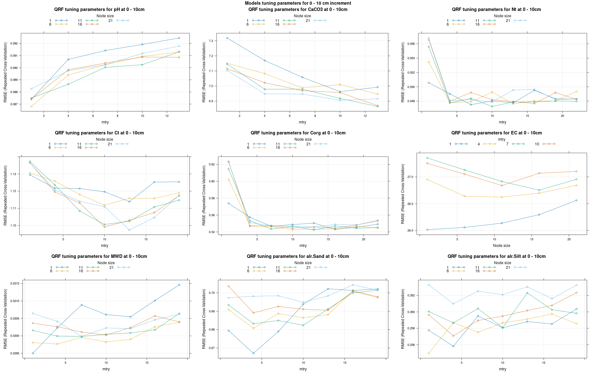
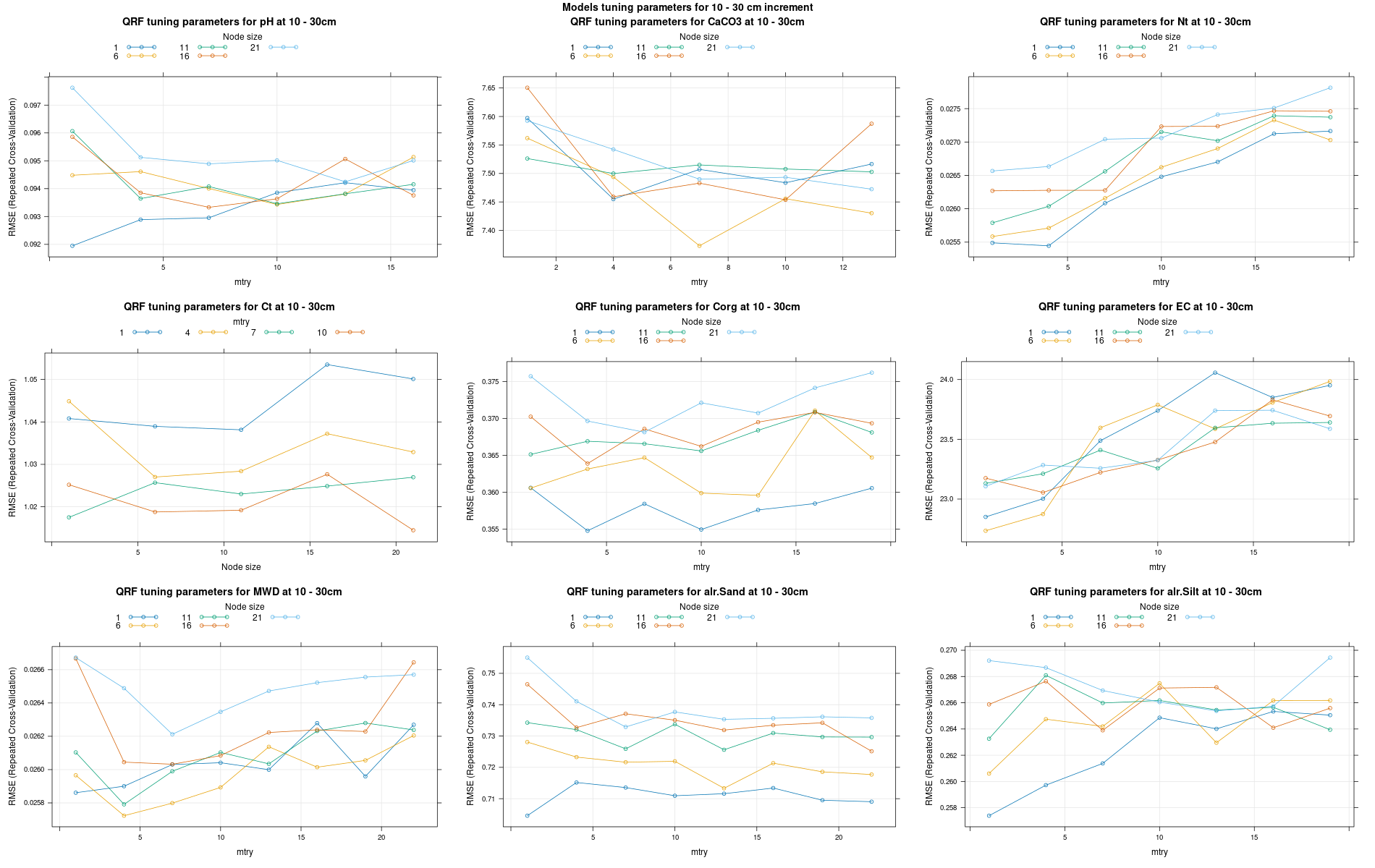
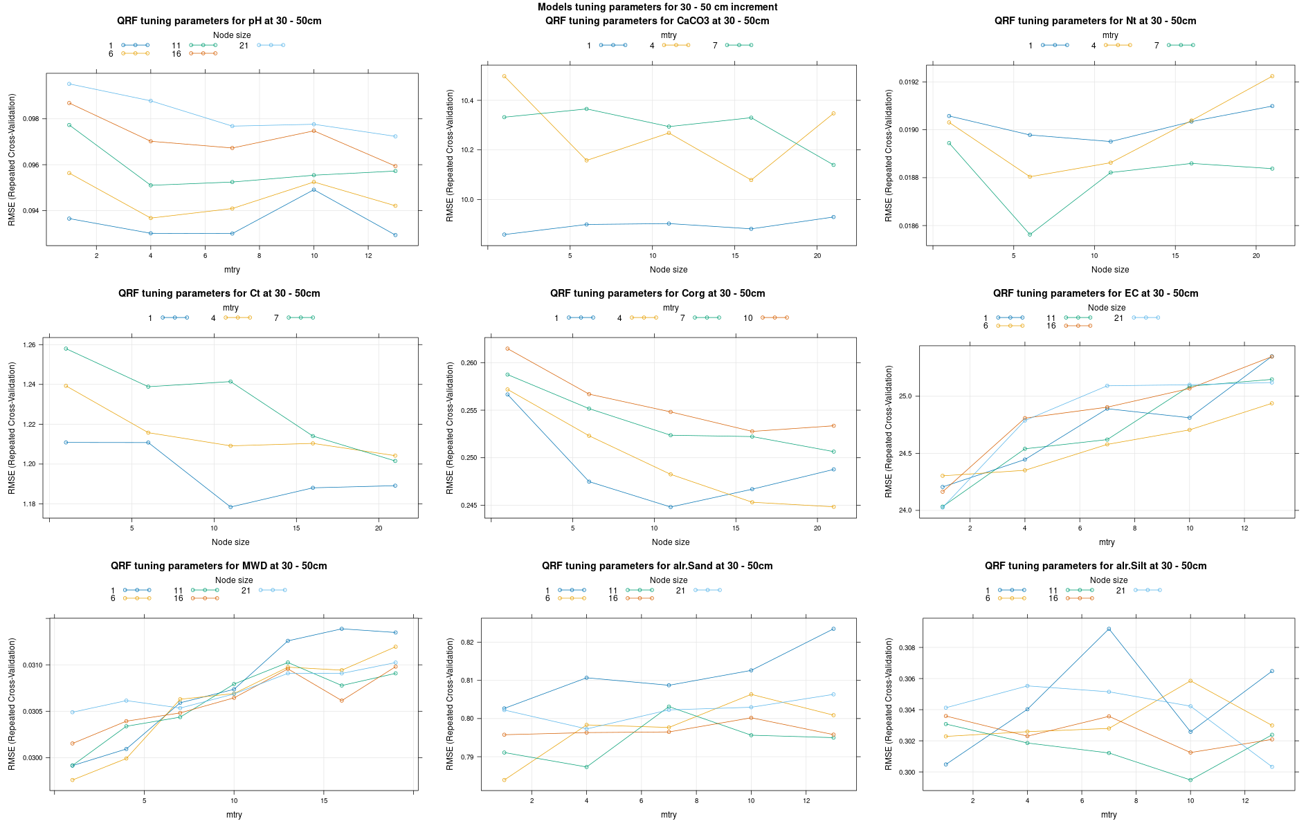
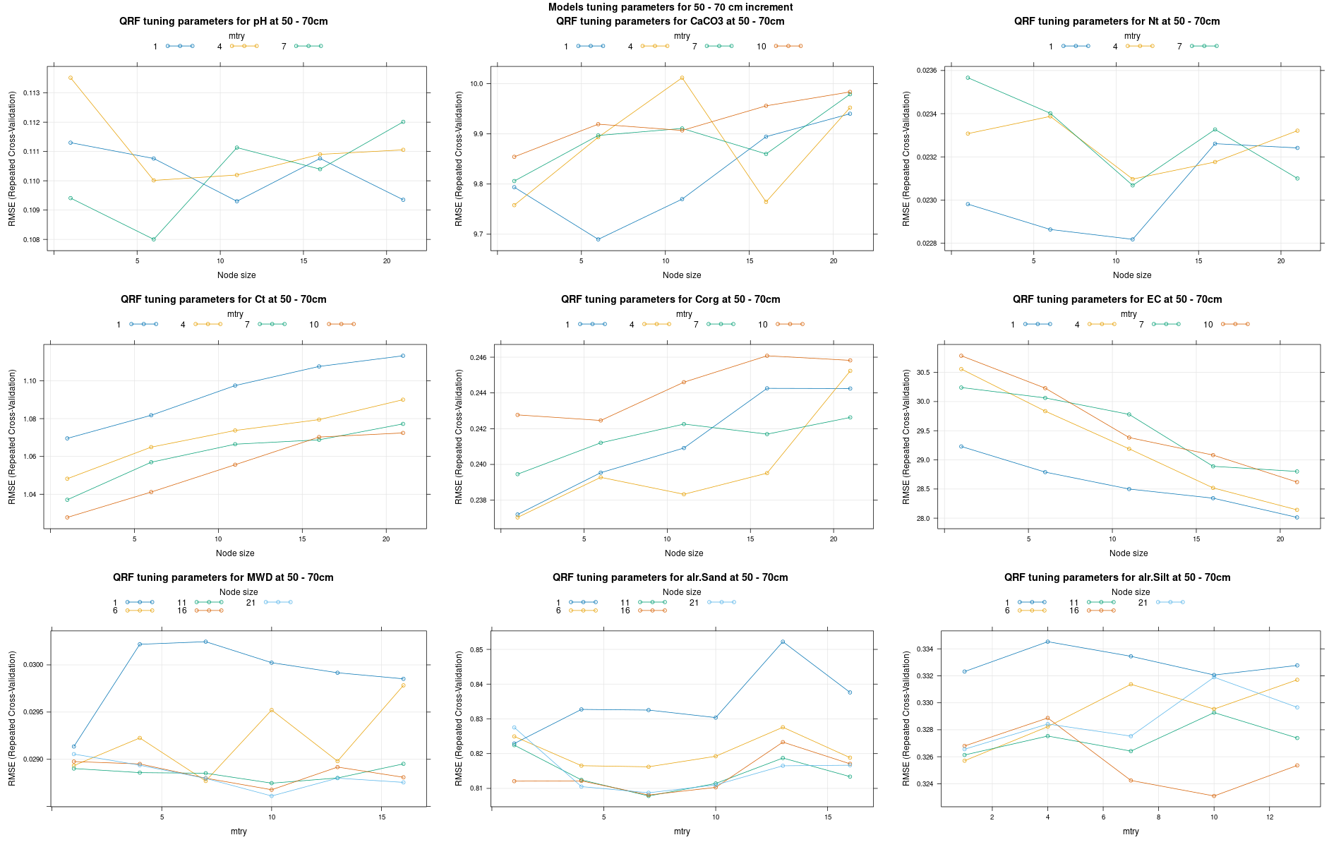
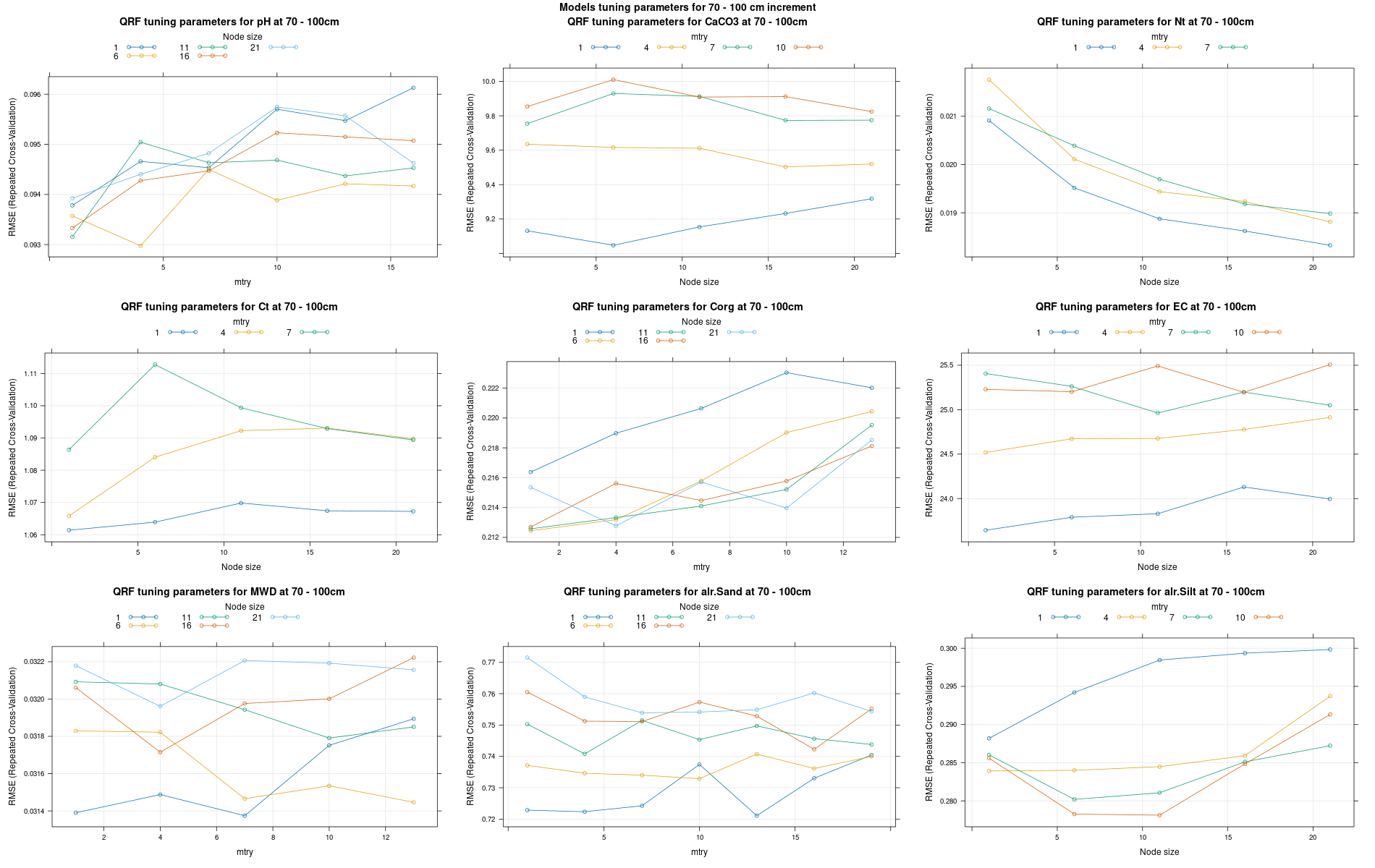
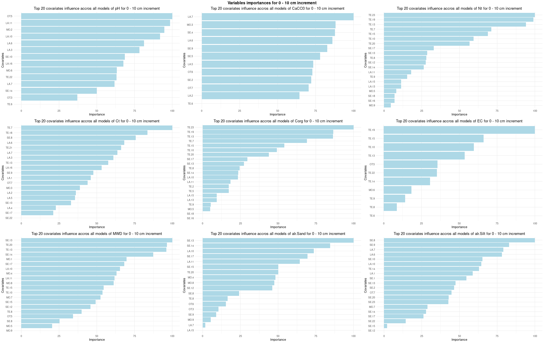
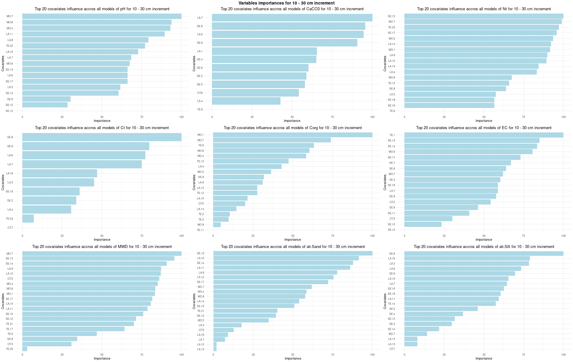
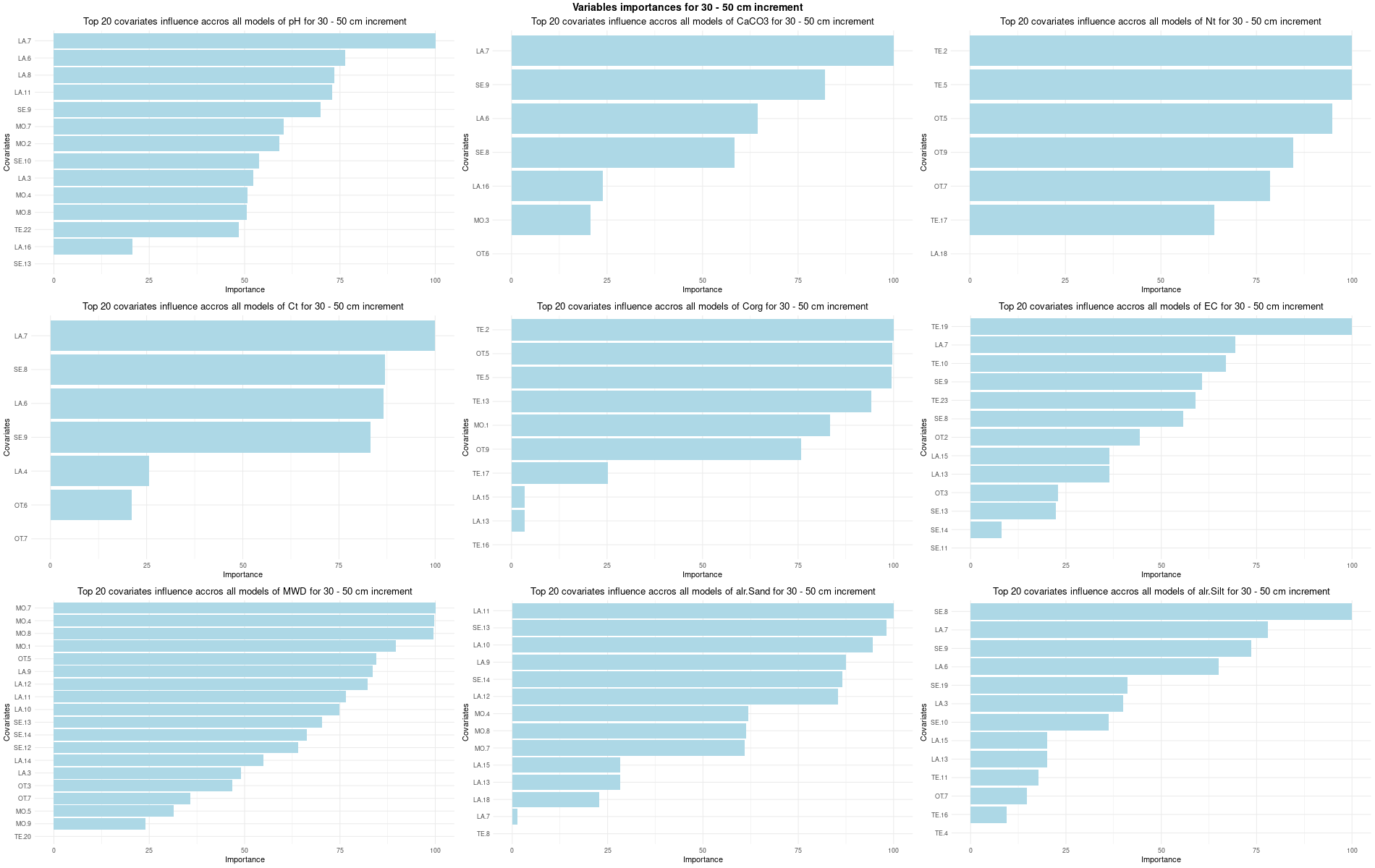
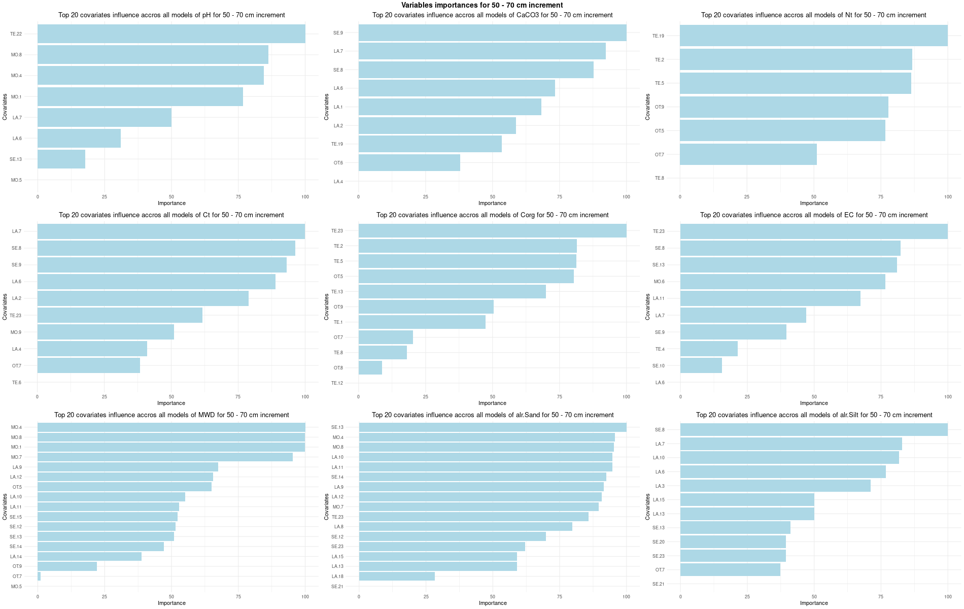
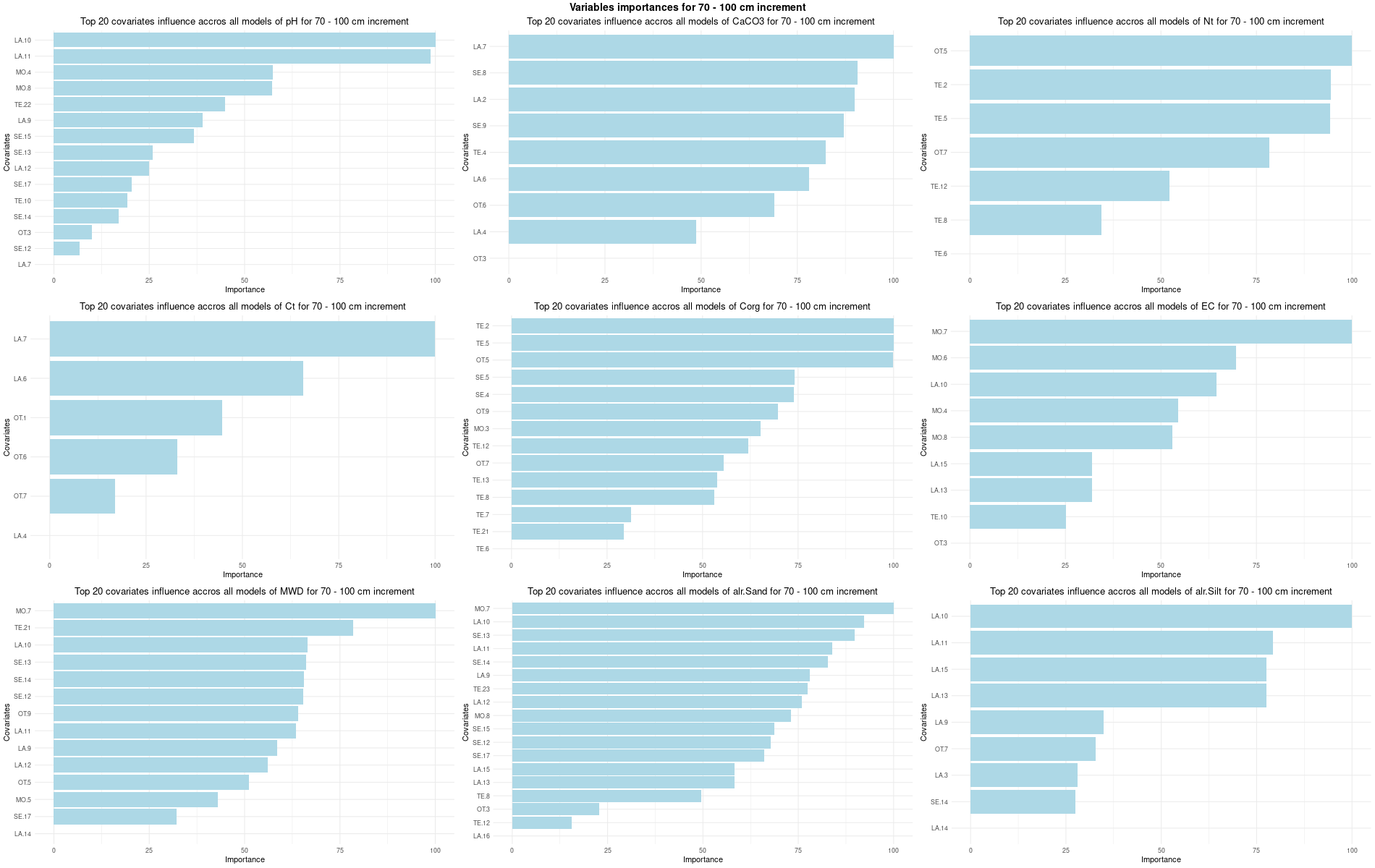
# 05. Variation of the models ##################################################
# 05.1 RFE =====================================================================

# Just replace Boruta by RFE for each element it is associated with

# 05.1 Split for the SoilGrid ==================================================
# Add this lines


split <- createDataPartition(SoilCovML[[1]][,length(SoilCovML[[1]])], p = 0.8, list = FALSE, times = 1)
Train_data <- lapply(SoilCovML, function(df) df[split, ])
Test_data  <- lapply(SoilCovML, function(df) df[-split, ])

Models[[depth]] <- list(
  Cov = SoilCovML,
  Models = FitQRaFCon,
  Metrics = metrics_final,
  Var_scores = var_importance,
  Models_plots = plot_list,
  Var_plots = VarPlots,
  Train_data = Train_data,
  Test_data = Test_data)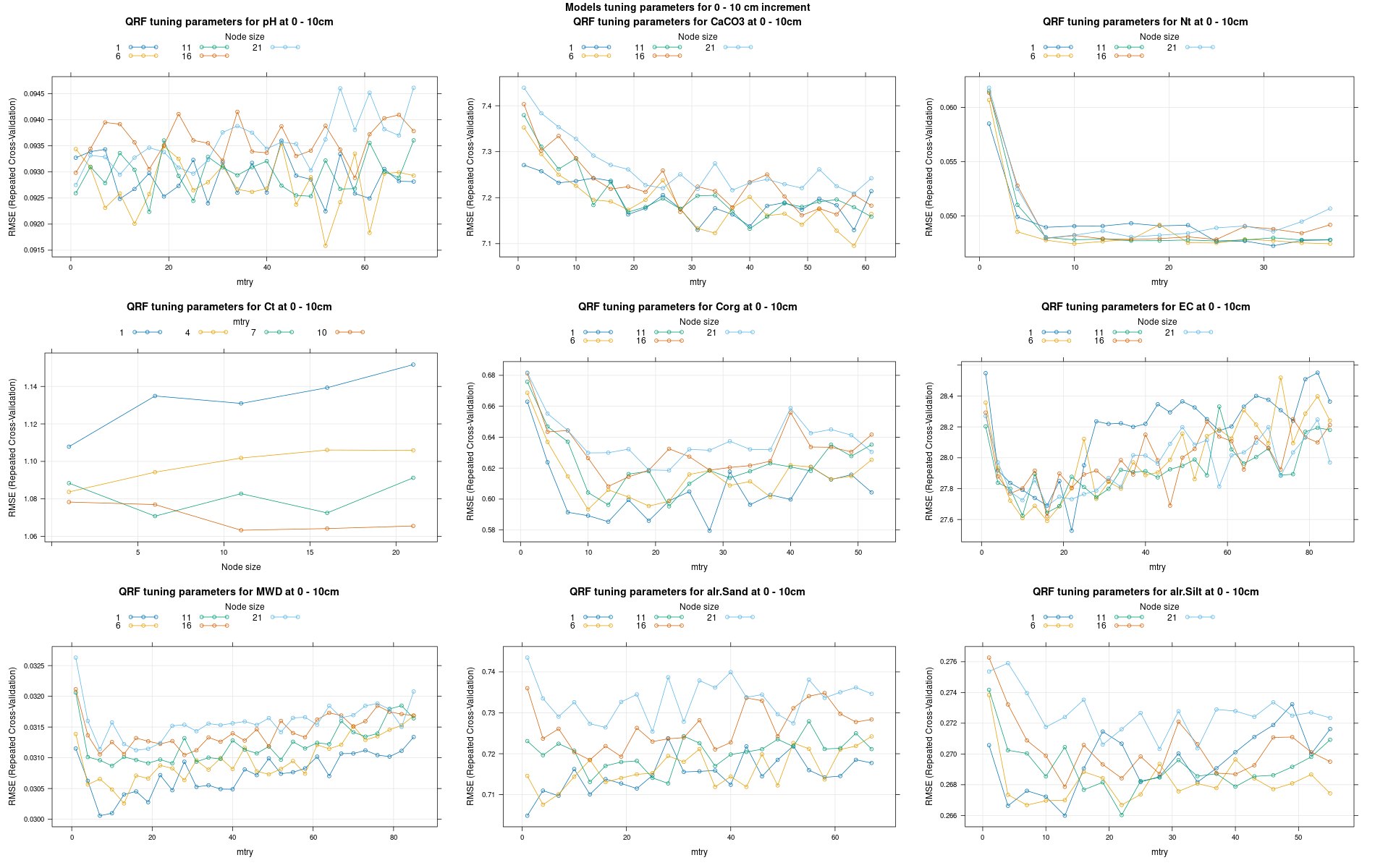
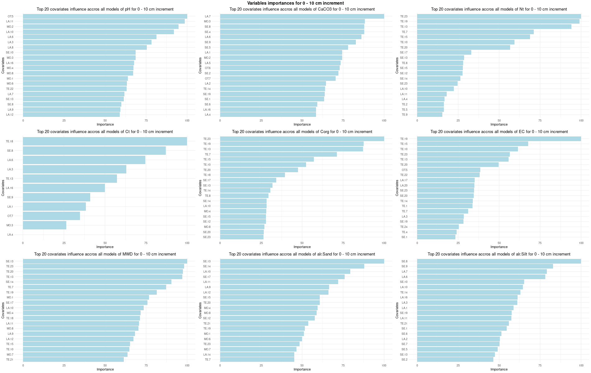
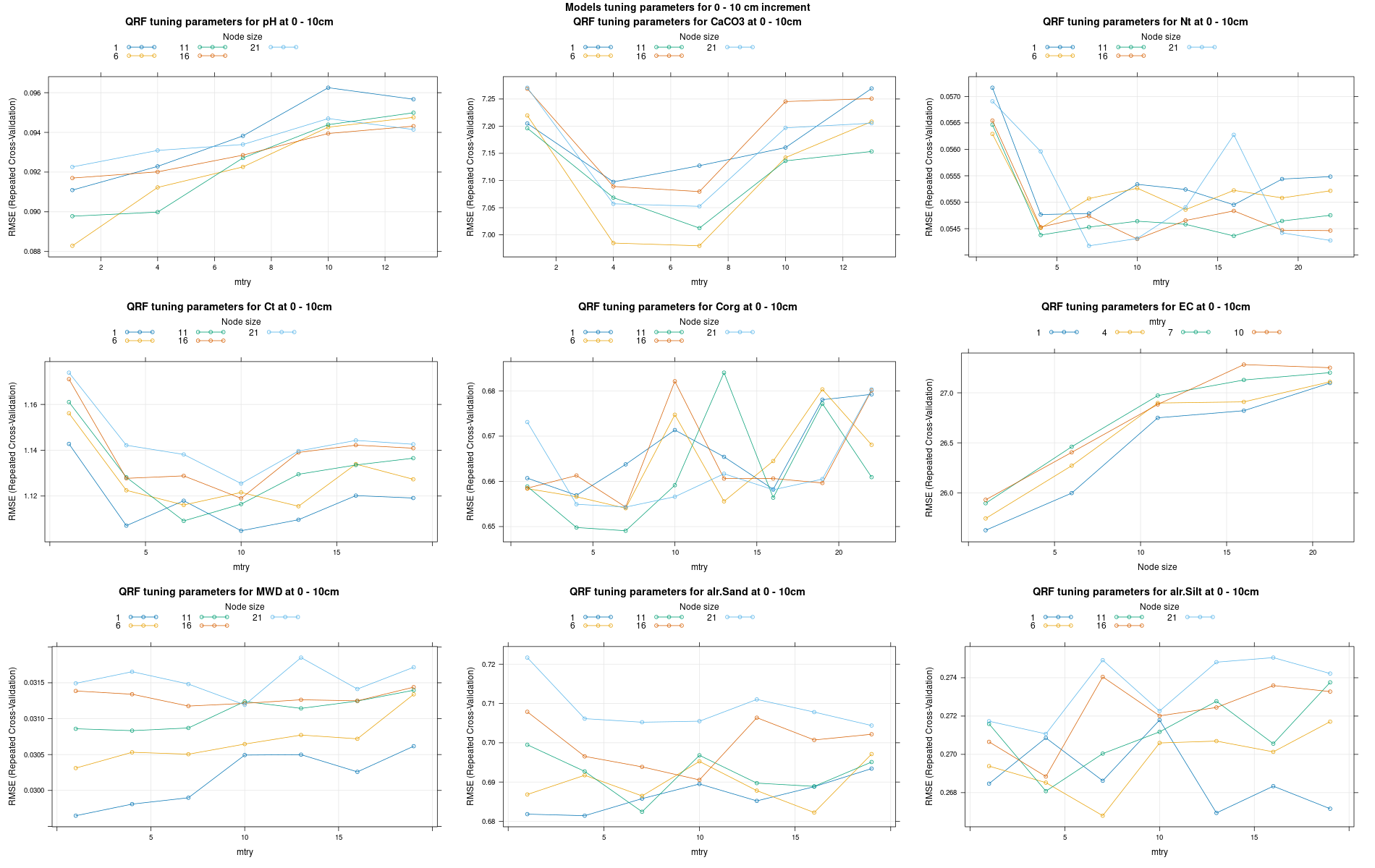
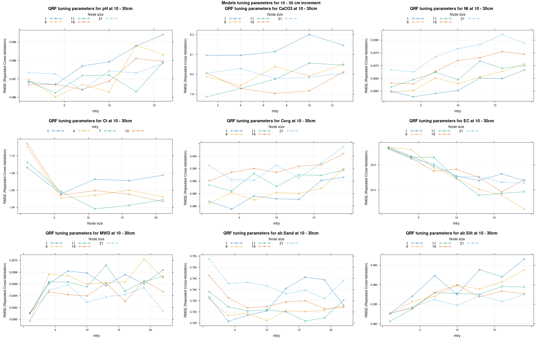
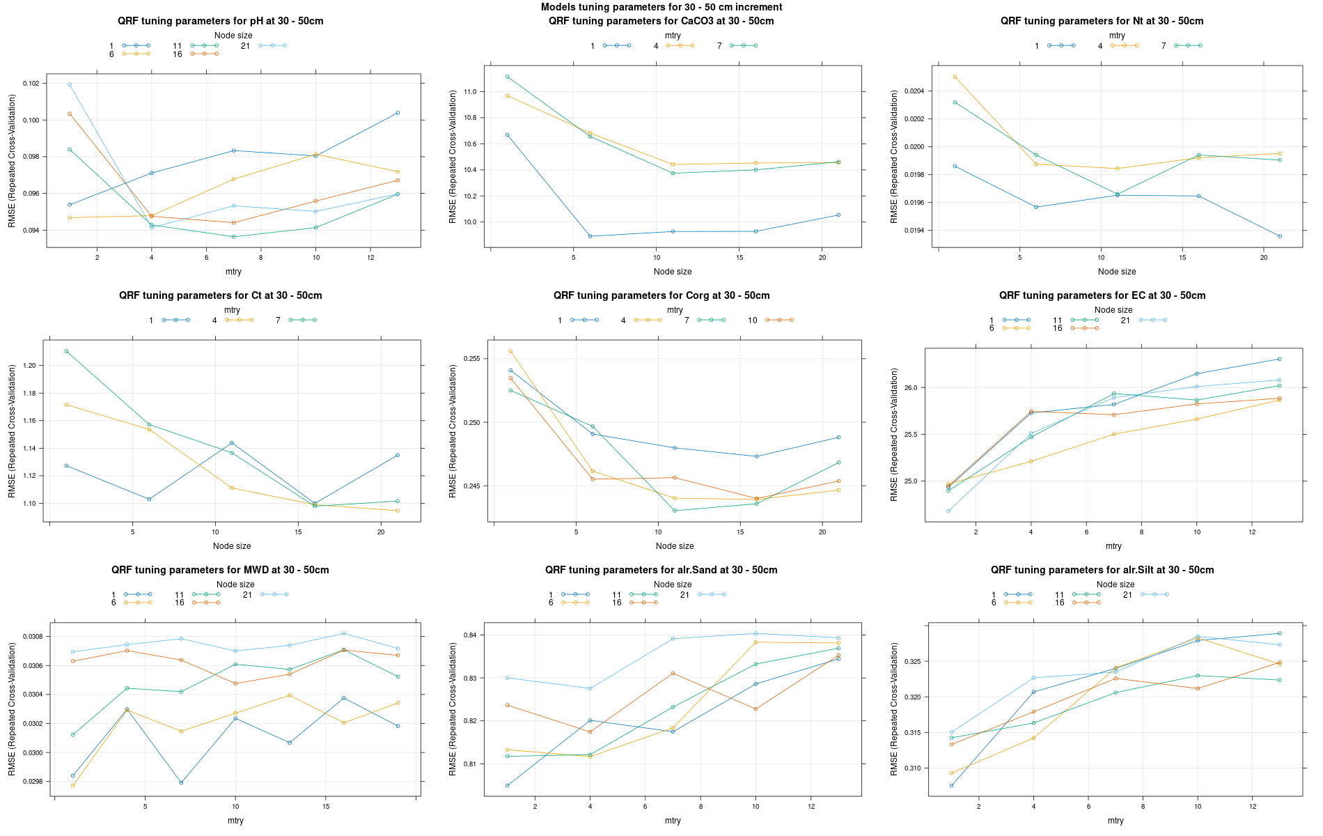
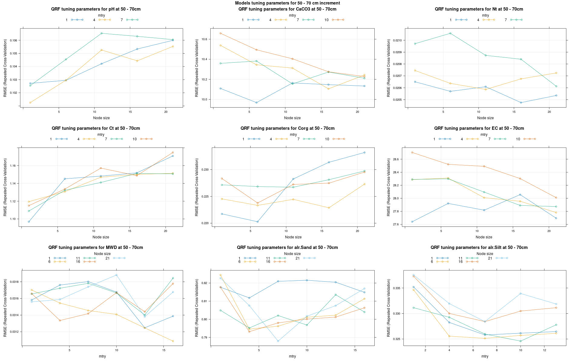
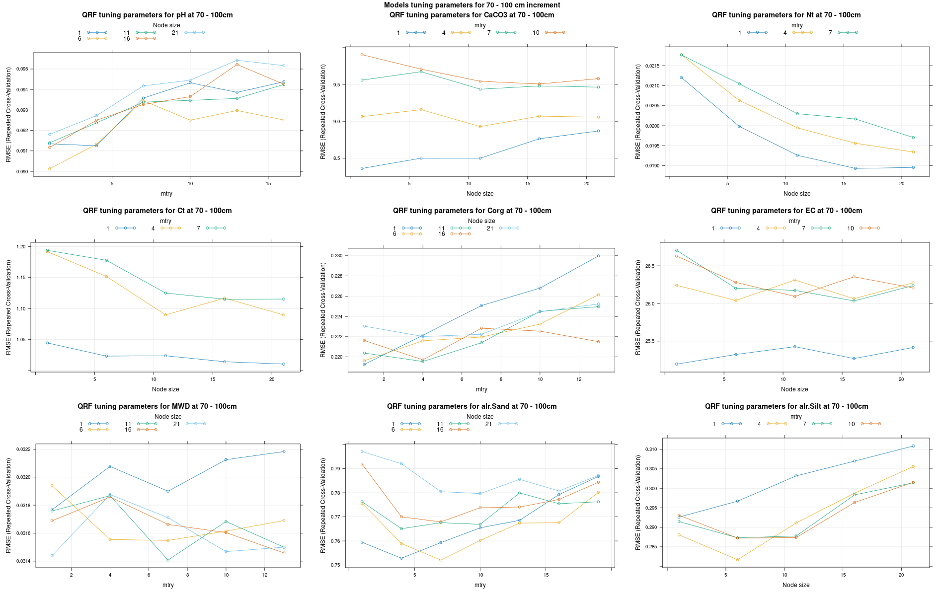
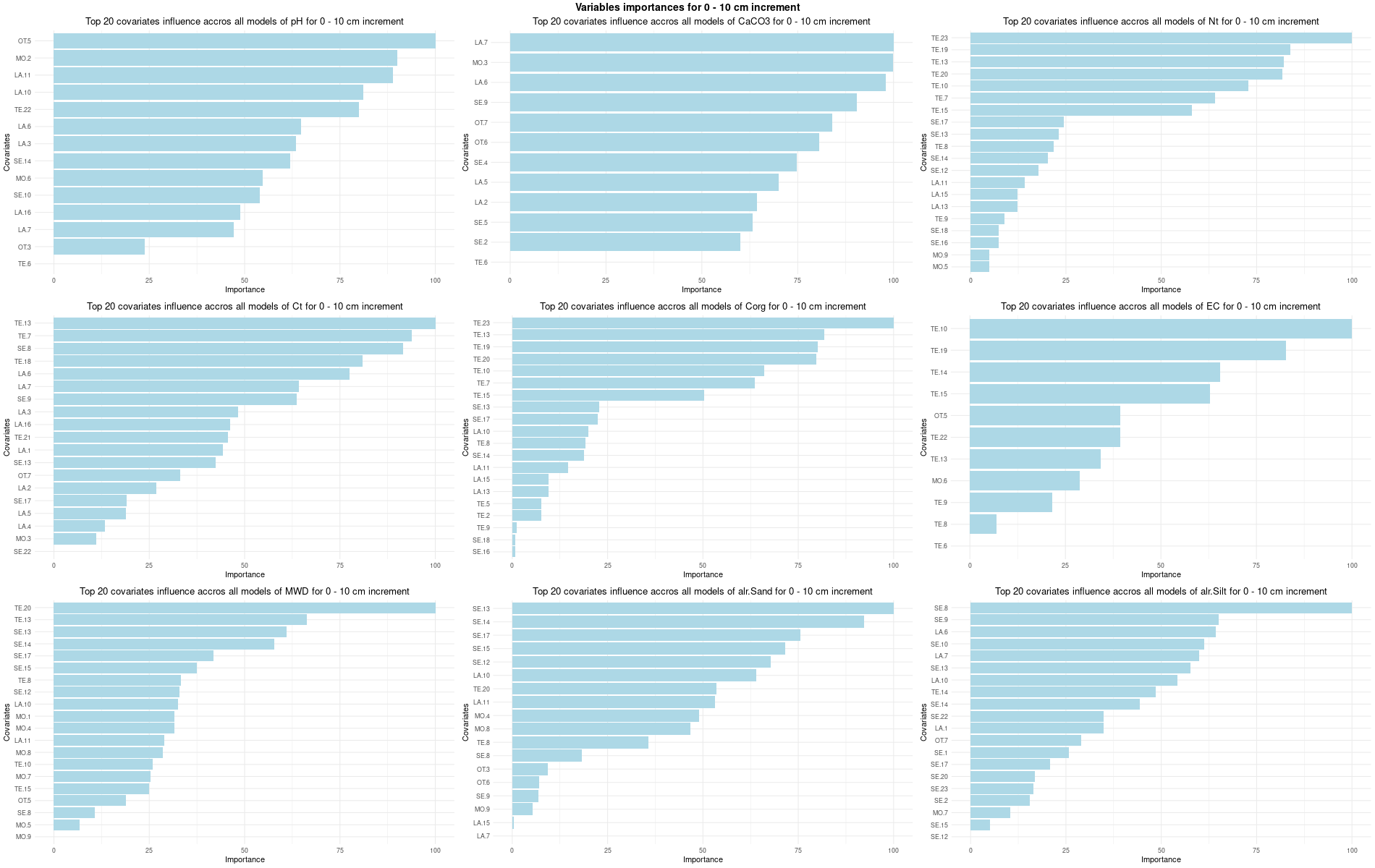
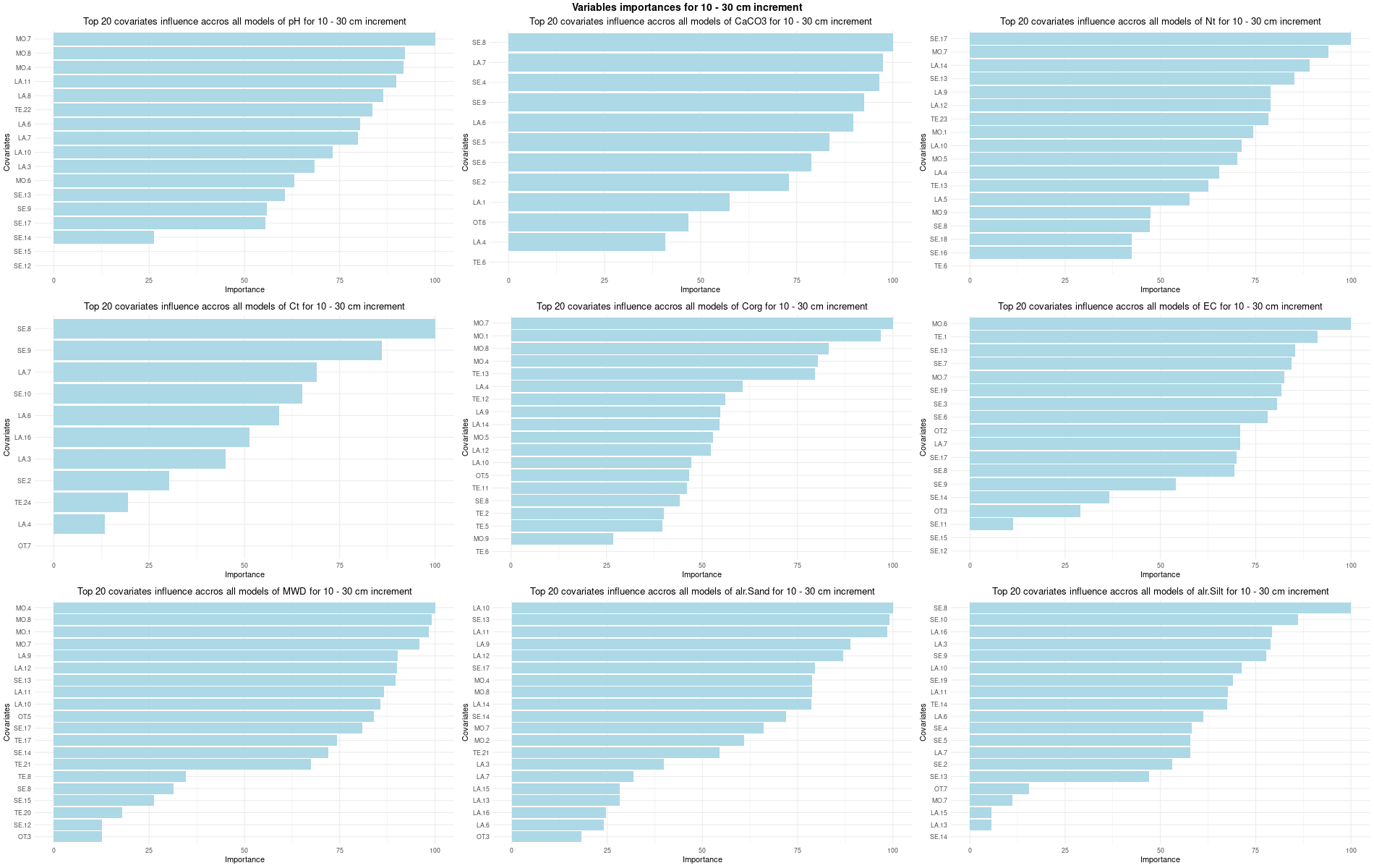
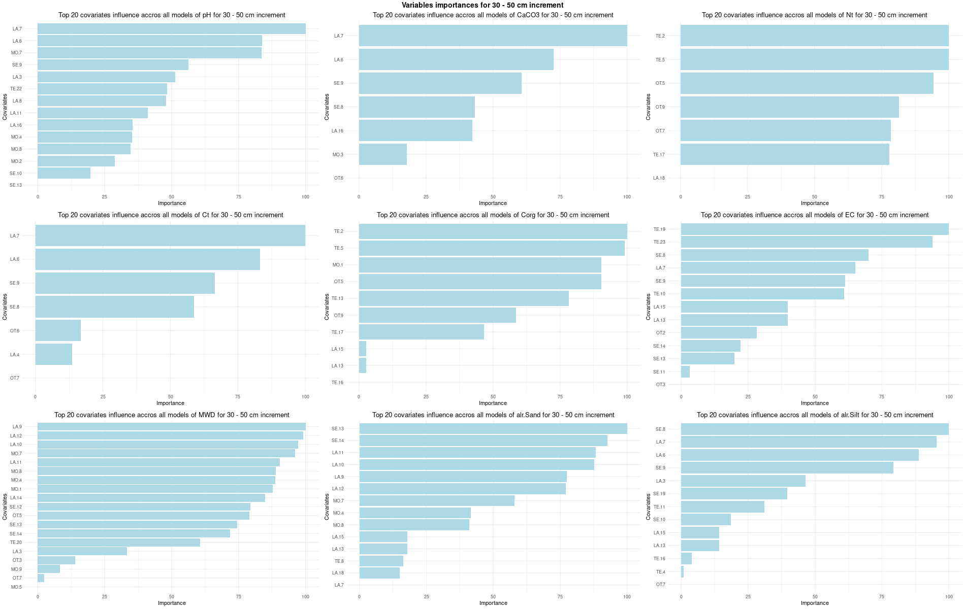
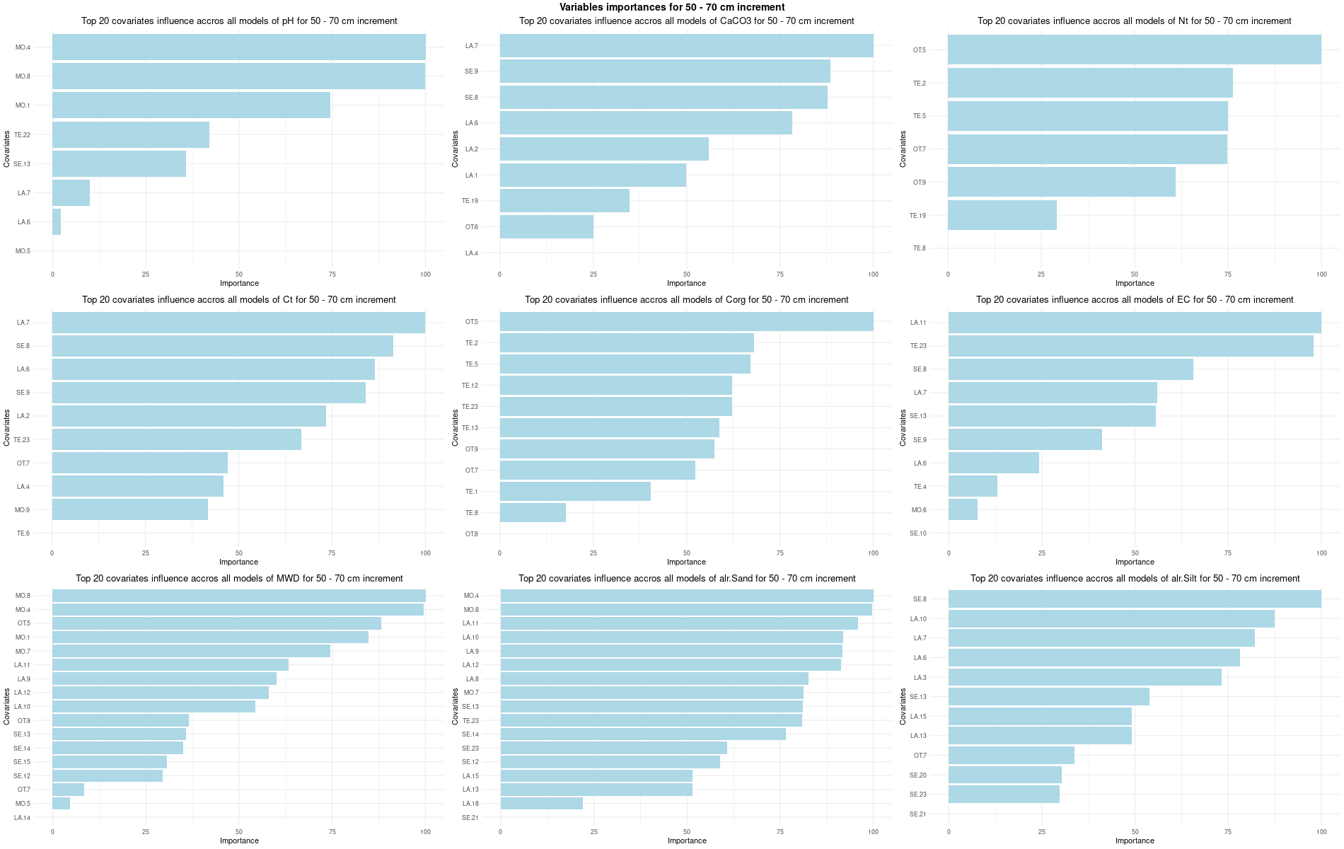
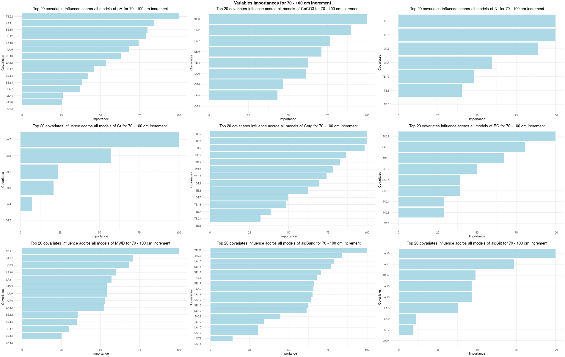
7.4 Model evaluation
We used four metrics to evaluate the model:
- ME = Bias with the mean error.
- RMSE = Root mean square error.
- R\(^2\) = Coefficient of determination, also called rsquared.
- PICP = Prediction interval coverage probability set at 90% interval
\[ \\[0.5cm] ME = \frac{1}{n} \sum_{i=n}^{n}(\hat{y}_i - y_i) \]
Where: \(n\) is the number of observations, \(y_i\) the observed value for \(i\), and \(\hat{y}_i\) the predicted value for \(i\).
\[ \\[0.5cm] RMSE = \sqrt{\frac{\sum_{i=1}^{n}(y_i - \hat{y}_i)^2}{N}} \]
Where: \(n\) is the number of observations, \(y_i\) the observed value for \(i\), and \(\hat{y}_i\) the predicted value for \(i\).
\[ \\[0.5cm] R^2 = 1 - \frac{\sum_{i=1}^{n}(y_i - \hat{y}_i)^2}{\sum_{i=1}^{n}(y_i - \bar{y}_i)^2} \]
Where: \(y_i\) the observed value for \(i\), \(\hat{y}_i\) the predicted value for \(i\), and \(\bar{y}\) is the mean of observed values.
\[ \\[0.5cm] PICP = \frac{1}{v} ~ count ~ j \\ j = PL^{L}_{j} \leq t_j \leq PL^{U}_{j} \]
Where: \(v\) is the number of observations, \(obs_i\) is the observed value for \(i\), \(PL^{L}_{i}\) is the lower prediction limit for \(i\), and \(PL^{U}_{i}\) is the upper prediction limit for \(i\).
7.4.1 Preparation of the environment
# 0 Environment setup ##########################################################

# 0.1 Prepare environment ======================================================

# Folder check
getwd()

# Set folder direction
setwd()

# Clean up workspace
rm(list = ls(all.names = TRUE))

# 0.2 Install packages =========================================================

install.packages("pacman")
#Install and load the "pacman" package (allow easier download of packages)
library(pacman)

pacman::p_load(ggplot2, DescTools, caret, grid, gridExtra, raster, readr, dplyr,
terra, quantregForest, compositions, cli, kableExtra, tidyr)## R version 4.5.3 (2026-03-11)
## Platform: x86_64-pc-linux-gnu
## Running under: EndeavourOS
##
## Matrix products: default
## BLAS: /usr/lib/libblas.so.3.12.0
## LAPACK: /usr/lib/liblapack.so.3.12.0 LAPACK version 3.12.0
##
## locale:
## [1] LC_CTYPE=fr_FR.UTF-8 LC_NUMERIC=C
## [3] LC_TIME=fr_FR.UTF-8 LC_COLLATE=fr_FR.UTF-8
## [5] LC_MONETARY=fr_FR.UTF-8 LC_MESSAGES=fr_FR.UTF-8
## [7] LC_PAPER=fr_FR.UTF-8 LC_NAME=C
## [9] LC_ADDRESS=C LC_TELEPHONE=C
## [11] LC_MEASUREMENT=fr_FR.UTF-8 LC_IDENTIFICATION=C
##
## time zone: Europe/Paris
## tzcode source: system (glibc)
##
## attached base packages:
## [1] grid stats graphics grDevices utils datasets methods
## [8] base
##
## other attached packages:
## [1] Boruta_9.0.0 raster_3.6-32 stars_0.7-1 abind_1.4-8
## [5] ggpubr_0.6.3 gridExtra_2.3 cowplot_1.2.0 viridis_0.6.5
## [9] viridisLite_0.4.3 wesanderson_0.3.7 corrplot_0.95 soiltexture_1.5.3
## [13] ggplot2_4.0.2 simplerspec_0.2.1 foreach_1.5.2 kableExtra_1.4.0
## [17] dplyr_1.2.0 sf_1.0-24 mapview_2.11.4 sp_2.2-1
## [21] tidyr_1.3.2 stringr_1.6.0 terra_1.8-93 DT_0.34.0
## [25] readr_2.2.0 bookdown_0.46 tufte_0.14.0 rmarkdown_2.30
## [29] knitr_1.51
##
## loaded via a namespace (and not attached):
## [1] RColorBrewer_1.1-3 rstudioapi_0.18.0 jsonlite_2.0.0
## [4] magrittr_2.0.4 farver_2.1.2 vctrs_0.7.1
## [7] base64enc_0.1-6 rstatix_0.7.3 htmltools_0.5.9
## [10] broom_1.0.12 pROC_1.19.0.1 Formula_1.2-5
## [13] caret_7.0-1 parallelly_1.46.1 sass_0.4.10
## [16] KernSmooth_2.23-26 bslib_0.10.0 htmlwidgets_1.6.4
## [19] plyr_1.8.9 lubridate_1.9.5 cachem_1.1.0
## [22] uuid_1.2-2 lifecycle_1.0.5 iterators_1.0.14
## [25] pkgconfig_2.0.3 Matrix_1.7-4 R6_2.6.1
## [28] fastmap_1.2.0 future_1.69.0 digest_0.6.39
## [31] patchwork_1.3.2 leafem_0.2.5 textshaping_1.0.4
## [34] crosstalk_1.2.2 labeling_0.4.3 timechange_0.4.0
## [37] compiler_4.5.3 proxy_0.4-29 bit64_4.6.0-1
## [40] withr_3.0.2 brew_1.0-10 S7_0.2.1
## [43] backports_1.5.0 carData_3.0-6 DBI_1.2.3
## [46] ggsignif_0.6.4 MASS_7.3-65 lava_1.8.2
## [49] leaflet_2.2.3 classInt_0.4-11 ModelMetrics_1.2.2.2
## [52] tools_4.5.3 units_1.0-0 otel_0.2.0
## [55] future.apply_1.20.2 nnet_7.3-20 glue_1.8.0
## [58] satellite_1.0.6 nlme_3.1-168 reshape2_1.4.5
## [61] generics_0.1.4 recipes_1.3.1 gtable_0.3.6
## [64] leaflet.providers_2.0.0 tzdb_0.5.0 class_7.3-23
## [67] data.table_1.18.2.1 hms_1.1.4 xml2_1.5.2
## [70] car_3.1-5 pillar_1.11.1 vroom_1.7.0
## [73] splines_4.5.3 lattice_0.22-9 survival_3.8-6
## [76] bit_4.6.0 tidyselect_1.2.1 svglite_2.2.2
## [79] stats4_4.5.3 xfun_0.56 hardhat_1.4.2
## [82] leafpop_0.1.0 timeDate_4052.112 stringi_1.8.7
## [85] yaml_2.3.12 evaluate_1.0.5 codetools_0.2-20
## [88] tcltk_4.5.3 tibble_3.3.1 cli_3.6.5
## [91] rpart_4.1.24 reticulate_1.45.0 systemfonts_1.3.1
## [94] jquerylib_0.1.4 Rcpp_1.1.1 globals_0.19.0
## [97] png_0.1-8 parallel_4.5.3 gower_1.0.2
## [100] listenv_0.10.0 ipred_0.9-15 scales_1.4.0
## [103] prodlim_2025.04.28 e1071_1.7-17 purrr_1.2.1
## [106] crayon_1.5.3 rlang_1.1.7# 06 Evaluation process of the models ##########################################
# Here we decided to split every run by soil depth to have a better vision
# on the running process.
# 06.1 Preparation =============================================================
make_subdir <- function(parent_dir, subdir_name) {
path <- file.path(parent_dir, subdir_name)
if (!dir.exists(path)) {
dir.create(path, recursive = TRUE)
message("✅ Folder created", path)
} else {
message("ℹ️ Existing folder : ", path)
}
return(path)
}
make_subdir("./export", "evaluation")
calc_cv <- function(x) {
(sd(x, na.rm = TRUE) / mean(x, na.rm = TRUE)) * 100
}
increments <- c("0_10", "10_30", "30_50", "50_70", "70_100")
load(file = "./export/save/Models_DSM_Boruta.RData")
Models_Boruta <- Models
load(file = "./export/save/Models_DSM_RFE.RData")
Models_RFE <- Models
# 06.2 Compare Boruta and RFE ==================================================
Metrics_diff <- data.frame()
Boruta_metrics <- Models_Boruta[[1]]$Metrics[,c(1:4)]
RFE_metrics <- Models_RFE[[1]]$Metrics[,c(1:4)]
Metrics_compared <- cbind(Boruta_metrics[,1], RFE_metrics[,1])
for (i in 2:4) {
Metrics_compared <- cbind(Metrics_compared, Boruta_metrics[,i], RFE_metrics[,i])
}
Metrics_compared <- as.data.frame(Metrics_compared)
metrics_names <- c("ME", "ME", "RMSE", "RMSE", "R2", "R2", "PICP", "PICP")
for (i in seq(1,7, by = 2)) {
colnames(Metrics_compared)[i] <- paste0("Boruta_",metrics_names[i])
}
for (i in seq(2,8, by = 2)) {
colnames(Metrics_compared)[i] <- paste0("RFE_",metrics_names[i])
}
Metrics_compared[,c(7:8)] <- Metrics_compared[,c(7:8)]*100
print(Metrics_compared)
write.csv(Metrics_compared, "./export/evaluation/Boruta_vs_RFE_0_10_metrics.csv")
# 06.3 Code for the table format (LaTEX) =======================================
cond1 <- abs(Metrics_compared[[1]]) < abs(Metrics_compared[[2]])
cond3 <- abs(Metrics_compared[[3]]) < abs(Metrics_compared[[4]])
cond5 <- abs(Metrics_compared[[5]] - 1) < abs(Metrics_compared[[6]] - 1)
cond7 <- abs(Metrics_compared[[7]] - 90) < abs(Metrics_compared[[8]] - 90)
Metrics_compared[[1]] <- ifelse(cond1,
cell_spec(Metrics_compared[[1]], "html", background = "lightgreen"),
as.character(Metrics_compared[[1]]))
Metrics_compared[[3]] <- ifelse(cond3,
cell_spec(Metrics_compared[[3]], "html", background = "lightgreen"),
as.character(Metrics_compared[[3]]))
Metrics_compared[[5]] <- ifelse(cond5,
cell_spec(Metrics_compared[[5]], "html", background = "lightgreen"),
as.character(Metrics_compared[[5]]))
Metrics_compared[[7]] <- ifelse(cond7,
cell_spec(Metrics_compared[[7]], "html", background = "lightgreen"),
as.character(Metrics_compared[[7]]))
kable(Metrics_compared, "html", escape = FALSE) %>%
kable_styling(full_width = FALSE) %>%
scroll_box(width = "100%")| X | Boruta_ME | RFE_ME | Boruta_RMSE | RFE_RMSE | Boruta_R2 | RFE_R2 | Boruta_PICP | RFE_PICP |
|---|---|---|---|---|---|---|---|---|
| 1 | -0.00187942818653847 | 0.0006730 | 0.0868006499212673 | 0.0915842 | 0.289926018165291 | 0.2270379 | 89.8717948717949 | 90.70513 |
| 2 | -0.0980560333547009 | -0.1552429 | 6.8648687718968 | 7.0952355 | 0.303002864996814 | 0.3116906 | 86.4529914529915 | 86.05922 |
| 3 | -0.0085645114534188 | -0.0071641 | 0.0472538299227664 | 0.0472469 | 0.448644085046708 | 0.5100507 | 87.7350427350427 | 87.74725 |
| 4 | -0.142084521164209 | -0.1331327 | 1.09745018242138 | 1.0632870 | 0.320053731800607 | 0.3400574 | 90.1495726495726 | 85.74786 |
| 5 | -0.109099969474969 | -0.1235417 | 0.542333065068082 | 0.5795000 | 0.491793749709384 | 0.4287227 | 87.7899877899878 | 86.92308 |
| 6 | 1.82203359095086 | 0.5972767 | 26.0150194154974 | 27.5271462 | 0.231145309646387 | 0.1818412 | 84.6794871794872 | 87.02991 |
| 7 | -0.00485160482773199 | -0.0049074 | 0.0295004399515017 | 0.0300581 | 0.386890856600006 | 0.3615785 | 88.7606837606838 | 89.91453 |
| 8 | -0.0989036968179061 | -0.1370804 | 0.667105040633794 | 0.7048553 | 0.440106001240199 | 0.3930319 | 87.0299145299145 | 89.59402 |
| 9 | -0.0235165354252422 | -0.0304478 | 0.254947790235202 | 0.2659848 | 0.351446997476728 | 0.2770322 | 90.4059829059829 | 88.22650 |
| 10 | -2.90751291737475 | -3.7092526 | 11.165902482486 | 11.7370619 | 0.43013935049469 | 0.3546744 | 73.1623931623932 | 79.20940 |
| 11 | 1.08662956313037 | 1.4211896 | 8.65081167702659 | 8.8865334 | 0.354706524120263 | 0.2662582 | 25.1282051282051 | 14.50855 |
| 12 | 1.82088335424438 | 2.2880630 | 6.85430844542249 | 7.1493428 | 0.378922510714082 | 0.3340440 | 0 | 0.00000 |
# 06.4 Full metrics for table format (LaTEX) ===================================

Metrics <- list()
for (depth in increments) {
  Metrics[[depth]] <- Models_Boruta[[depth]]$Metrics[,c(1:4)]
  Metrics[[depth]][,4] <- Metrics[[depth]][,4]*100
  colnames(Metrics[[depth]]) <- c("ME", "RMSE", "R2", "PCIP")

}

Metrics <- lapply(Metrics, function(df){
  df %>%
    mutate(Variable = rownames(.))
})

Metrics <- lapply(names(Metrics), function(name){

  Metrics[[name]] %>%
    pivot_longer(
      cols = -Variable,
      names_to = "Metric",
      values_to = "Value"
    ) %>%
    mutate(Profondeur = name)

})

final_metrics <- bind_rows(Metrics)


final_metrics <- final_metrics %>%
  pivot_wider(
    names_from = Profondeur,
    values_from = Value
  ) %>%
  arrange(Variable, Metric)

final_metrics[,c(3:7)] <- round(final_metrics[,c(3:7)], digit = 2)

# Change the "html" to "latex"
kable(final_metrics, "html", escape = FALSE) %>%
  kable_styling(full_width = FALSE) %>%
scroll_box(width = "100%")| Variable | Metric | 0_10 | 10_30 | 30_50 | 50_70 | 70_100 |
|---|---|---|---|---|---|---|
| CaCO3 | ME | -0.10 | -0.41 | -0.90 | -1.26 | -1.80 |
| CaCO3 | PCIP | 86.45 | 84.07 | 87.38 | 89.33 | 85.58 |
| CaCO3 | R2 | 0.30 | 0.32 | 0.27 | 0.33 | 0.20 |
| CaCO3 | RMSE | 6.86 | 7.37 | 9.86 | 9.69 | 9.05 |
| Clay | ME | 1.82 | 2.34 | 2.17 | 1.75 | 1.78 |
| Clay | PCIP | 0.00 | 0.00 | 0.00 | 0.00 | 0.00 |
| Clay | R2 | 0.38 | 0.34 | 0.29 | 0.30 | 0.40 |
| Clay | RMSE | 6.85 | 6.88 | 7.68 | 8.04 | 7.54 |
| Corg | ME | -0.11 | -0.07 | -0.03 | -0.04 | -0.04 |
| Corg | PCIP | 87.79 | 88.18 | 88.46 | 85.45 | 90.76 |
| Corg | R2 | 0.49 | 0.37 | 0.37 | 0.44 | 0.43 |
| Corg | RMSE | 0.54 | 0.35 | 0.24 | 0.24 | 0.21 |
| Ct | ME | -0.14 | -0.04 | -0.20 | -0.13 | -0.11 |
| Ct | PCIP | 90.15 | 89.24 | 89.81 | 83.61 | 84.24 |
| Ct | R2 | 0.32 | 0.39 | 0.33 | 0.34 | 0.23 |
| Ct | RMSE | 1.10 | 1.01 | 1.18 | 1.03 | 1.06 |
| EC | ME | 1.82 | 0.58 | 2.92 | 4.83 | 1.11 |
| EC | PCIP | 84.68 | 91.77 | 89.32 | 90.83 | 87.04 |
| EC | R2 | 0.23 | 0.30 | 0.31 | 0.22 | 0.30 |
| EC | RMSE | 26.02 | 22.74 | 24.03 | 28.01 | 23.64 |
| MWD | ME | 0.00 | 0.00 | -0.01 | -0.01 | -0.01 |
| MWD | PCIP | 88.76 | 86.65 | 86.72 | 88.70 | 85.04 |
| MWD | R2 | 0.39 | 0.44 | 0.37 | 0.39 | 0.29 |
| MWD | RMSE | 0.03 | 0.03 | 0.03 | 0.03 | 0.03 |
| Nt | ME | -0.01 | 0.00 | 0.00 | 0.00 | 0.00 |
| Nt | PCIP | 87.74 | 87.75 | 87.26 | 86.87 | 89.53 |
| Nt | R2 | 0.45 | 0.36 | 0.29 | 0.22 | 0.24 |
| Nt | RMSE | 0.05 | 0.03 | 0.02 | 0.02 | 0.02 |
| Sand | ME | -2.91 | -3.35 | -2.93 | -3.26 | -3.08 |
| Sand | PCIP | 73.16 | 82.32 | 80.01 | 79.65 | 69.66 |
| Sand | R2 | 0.43 | 0.49 | 0.28 | 0.35 | 0.44 |
| Sand | RMSE | 11.17 | 9.90 | 11.15 | 11.98 | 10.97 |
| Silt | ME | 1.09 | 1.01 | 0.77 | 1.51 | 1.30 |
| Silt | PCIP | 25.13 | 26.53 | 20.95 | 29.82 | 24.03 |
| Silt | R2 | 0.35 | 0.43 | 0.29 | 0.25 | 0.38 |
| Silt | RMSE | 8.65 | 7.76 | 9.13 | 10.02 | 8.54 |
| alr.Sand | ME | -0.10 | -0.12 | -0.08 | -0.10 | -0.13 |
| alr.Sand | PCIP | 87.03 | 88.74 | 88.06 | 89.36 | 85.41 |
| alr.Sand | R2 | 0.44 | 0.47 | 0.32 | 0.41 | 0.45 |
| alr.Sand | RMSE | 0.67 | 0.70 | 0.78 | 0.81 | 0.72 |
| alr.Silt | ME | -0.02 | -0.04 | -0.04 | -0.02 | -0.02 |
| alr.Silt | PCIP | 90.41 | 88.89 | 89.03 | 89.11 | 87.95 |
| alr.Silt | R2 | 0.35 | 0.34 | 0.31 | 0.32 | 0.40 |
| alr.Silt | RMSE | 0.25 | 0.26 | 0.30 | 0.32 | 0.28 |
| pH | ME | 0.00 | -0.01 | 0.00 | -0.01 | -0.01 |
| pH | PCIP | 89.87 | 86.17 | 86.31 | 84.17 | 86.56 |
| pH | R2 | 0.29 | 0.30 | 0.37 | 0.33 | 0.29 |
| pH | RMSE | 0.09 | 0.09 | 0.09 | 0.11 | 0.09 |
# 06.5 Best tune ===============================================================

Tune_table <- list()
for (depth in increments) {
  depth_name <- gsub("_", "-", depth)
  depth_name <- paste0(depth_name, " cm")

  variables <- names(Models_Boruta[[depth]]$Models)
  for (variable in variables) {
    df <- cbind(variable, depth_name)
    df <- cbind(df, Models_Boruta[[depth]]$Models[[variable]]$bestTune)
    Tune_table[[depth]][[variable]] <- rbind(Tune_table[[depth]][[variable]], df)
  }
}

Tune_df <- lapply(1:9, function(i) {
  do.call(rbind, lapply(Tune_table, `[[`, i))
})

Tune_df <- do.call(rbind, Tune_df)

row.names(Tune_df) <- NULL

# Change the "html" to "latex"
kable(Tune_df, "html", escape = FALSE) %>%
  kable_styling(full_width = FALSE) %>%
  scroll_box(width = "100%")
7.5 Prediction of the area
Due to the highly detailed data we had to split the prediction into different blocks. This process allows the computer to run separately each prediction.
The uncertainty of the model is based on the following equation from Yan et al. (2018).
\[ \\[0.5cm] Uncertainty = \frac{Qp ~ 0.95- Qp ~ 0.05}{Qp ~ 0.5} \]
# 07 Prediction map for DSM ####################################################


# 07.1 Prediction loop  ========================================================

cl <- makeCluster(6)
registerDoParallel(cl)

for (depth in increments) {
  make_subdir("./export/prediction_DSM", depth)
  model_depth <- Models[[depth]]$Models

  cli_progress_bar(
    format =  " {.val {depth}}, {.val {variable}} {cli::pb_bar} {cli::pb_percent} [{cli::pb_current}/{cli::pb_total}] | ETA: {cli::pb_eta} - Elapsed: {cli::pb_elapsed_clock}",
    total = length(Models[[1]]$Models),
    clear = TRUE
  )

  for (i in 1:length(model_depth)) {

    variable <- colnames(Models[[depth]]$Cov[[i]][ncol(Models[[depth]]$Cov[[i]])])
    cov_names <- colnames(model_depth[[i]]$trainingData[,-1])
    rast <- covariates[[cov_names]]
    cov_df <- as.data.frame(rast, xy = TRUE)
    cov_df[is.infinite(as.matrix(cov_df))] <- NA
    cov_df <- na.omit(cov_df)

    n_blocks <- 10
    cov_df$block <- cut(1:nrow(cov_df), breaks = n_blocks, labels = FALSE)
    cov_df_blocks <- split(cov_df, cov_df$block)

    pred_model <- model_depth[[i]]$finalModel
    predicted_blocks <- list()

    # Create a loop for blocks
    for (j in 1:10) {
      block <- cov_df_blocks[[j]][,cov_names]
      prediction <- predict(pred_model, newdata = block,  what = c(0.05, 0.5, 0.95))

      # Write the predicted block to the output raster
      values <- prediction[,2]
      uncertainty <- (prediction[,3] - prediction[,1]) /prediction[,2]
      predicted_df <- cov_df_blocks[[j]][,c(1:2)]
      predicted_df$prediction <- values
      predicted_df$uncertainty <- uncertainty
      predicted_blocks[[j]] <- predicted_df
    }

    predicted_rast <- do.call(rbind,predicted_blocks)
    predicted_rast <- rast(predicted_rast, type ="xyz")
    crs(predicted_rast) <- crs(rast)
    writeRaster(predicted_rast, paste0("./export/prediction_DSM/",depth,"/Prediction_map_",variable,"_for_",depth,"_soil.tif"), overwrite = TRUE)
    cli_progress_update()
  }
  cli_progress_done()
}
7.6 Visualisation and comparison with SoilGrid product
7.6.1 Preparation of the environment
# 0.1 Prepare environment ======================================================

# Folder check
getwd()

# Set folder direction
setwd(dir="./depth")

# Clean up workspace
rm(list = ls(all.names = TRUE))

# 0.2 Install packages =========================================================

install.packages("pacman")        #Install and load the "pacman" package (allow easier download of packages)
library(pacman)

pacman::p_load(terra, sf, sp, viridis, ggplot2, DescTools, remotes, RColorBrewer, wesanderson, dplyr,
               grid, cli, caret, tidyr, kableExtra, gridExtra, colorspace, mapview, biscale, ncdf4,
               purrr, SpaDES, ggspatial,soiltexture, cowplot, hrbrthemes, compositions, quantregForest)

devtools::install_github("ducciorocchini/cblindplot")
library(cblindplot)

# 0.3 Show session infos =======================================================
R version 4.5.1 (2025-06-13 ucrt)
Platform: x86_64-w64-mingw32/x64
Running under: Windows 11 x64 (build 26200)
Matrix products: default
LAPACK version 3.12.1
locale:
[1] LC_COLLATE=French_France.utf8 LC_CTYPE=French_France.utf8 LC_MONETARY=French_France.utf8 LC_NUMERIC=C
[5] LC_TIME=French_France.utf8
time zone: Europe/Paris
tzcode source: internal
attached base packages:
[1] grid parallel stats graphics grDevices utils datasets methods base
other attached packages:
[1] cblindplot_0.0.4 quantregForest_1.3-7.1 randomForest_4.7-1.2 compositions_2.0-9 hrbrthemes_0.8.7 cowplot_1.2.0
[7] soiltexture_1.5.3 ggspatial_1.1.10 SpaDES.tools_2.1.1 SpaDES.core_3.0.4 quickPlot_1.0.4 reproducible_3.0.0
[13] SpaDES_2.0.11 purrr_1.2.1 ncdf4_1.24 biscale_1.1.0 mapview_2.11.4 colorspace_2.1-2
[19] gridExtra_2.3 kableExtra_1.4.0 tidyr_1.3.2 caret_7.0-1 lattice_0.22-7 cli_3.6.5
[25] dplyr_1.1.4 wesanderson_0.3.7 RColorBrewer_1.1-3 remotes_2.5.0 DescTools_0.99.60 ggplot2_4.0.1
[31] viridis_0.6.5 viridisLite_0.4.2 sp_2.2-0 sf_1.0-24 terra_1.8-93
loaded via a namespace (and not attached):
[1] splines_4.5.1 tibble_3.3.1 cellranger_1.1.0 hardhat_1.4.2 pROC_1.19.0.1 rpart_4.1.24
[7] lifecycle_1.0.5 tcltk_4.5.1 globals_0.18.0 MASS_7.3-65 crosstalk_1.2.2 backports_1.5.0
[13] magrittr_2.0.4 rmarkdown_2.30 yaml_2.3.12 otel_0.2.0 lobstr_1.1.3 gld_2.6.8
[19] bayesm_3.1-7 DBI_1.2.3 lubridate_1.9.4 expm_1.0-0 nnet_7.3-20 tensorA_0.36.2.1
[25] ipred_0.9-15 gdtools_0.4.4 satellite_1.0.6 lava_1.8.2 listenv_0.10.0 units_1.0-0
[31] parallelly_1.46.1 svglite_2.2.2 codetools_0.2-20 xml2_1.5.2 Require_1.0.1 tidyselect_1.2.1
[37] raster_3.6-32 farver_2.1.2 stats4_4.5.1 base64enc_0.1-3 e1071_1.7-17 survival_3.8-6
[43] iterators_1.0.14 systemfonts_1.3.1 foreach_1.5.2 tools_4.5.1 Rcpp_1.1.1 glue_1.8.0
[49] Rttf2pt1_1.3.14 prodlim_2025.04.28 qs2_0.1.7 xfun_0.56 withr_3.0.2 fastmap_1.2.0
[55] boot_1.3-32 digest_0.6.39 timechange_0.3.0 R6_2.6.1 textshaping_1.0.4 dichromat_2.0-0.1
[61] generics_0.1.4 fontLiberation_0.1.0 data.table_1.18.0 recipes_1.3.1 robustbase_0.99-6 class_7.3-23
[67] httr_1.4.7 htmlwidgets_1.6.4 whisker_0.4.1 ModelMetrics_1.2.2.2 pkgconfig_2.0.3 gtable_0.3.6
[73] Exact_3.3 timeDate_4051.111 rsconnect_1.7.0 S7_0.2.1 sys_3.4.3 htmltools_0.5.9
[79] fontBitstreamVera_0.1.1 bookdown_0.46 scales_1.4.0 lmom_3.2 png_0.1-8 gower_1.0.2
[85] knitr_1.51 rstudioapi_0.18.0 tzdb_0.5.0 reshape2_1.4.5 checkmate_2.3.3 nlme_3.1-168
[91] proxy_0.4-29 stringr_1.6.0 rootSolve_1.8.2.4 KernSmooth_2.23-26 extrafont_0.20 pillar_1.11.1
[97] vctrs_0.7.0 stringfish_0.18.0 extrafontdb_1.1 evaluate_1.0.5 readr_2.1.6 mvtnorm_1.3-3
[103] compiler_4.5.1 rlang_1.1.7 future.apply_1.20.1 classInt_0.4-11 plyr_1.8.9 forcats_1.0.1
[109] fs_1.6.6 stringi_1.8.7 fpCompare_0.2.4 leaflet_2.2.3 fontquiver_0.2.1 pacman_0.5.1
[115] Matrix_1.7-4 hms_1.1.4 leafem_0.2.5 future_1.69.0 haven_2.5.5 igraph_2.2.1
[121] RcppParallel_5.1.11-1 DEoptimR_1.1-4 readxl_1.4.5 7.6.2 Visualisation of the final products
Visualisations of the final products can also be reached on Shiny app website at https://mathias-bellat.shinyapps.io/Northern-Kurdistan-map/.
# 08 Prepare visualisations  ###################################################
# Here we decided to split every run by soil depth to have a better vision
# on the running process.
# 08.1 Prepare data ============================================================

make_subdir <- function(parent_dir, subdir_name) {
  path <- file.path(parent_dir, subdir_name)

  if (!dir.exists(path)) {
    dir.create(path, recursive = TRUE)
    message("✅  Folder created", path)
  } else {
    message("ℹ️ Existing folder : ", path)
  }

  return(path)
}
make_subdir("./export", "visualisations")
make_subdir("./export", "final_maps")

DEM <- rast("./data/Stack_layers_DSM.tif")
DEM <- DEM$TE.5
survey <- st_read("./data/Survey_Area.gpkg", layer = "Survey_Area")

increments <- c("0_10", "10_30", "30_50", "50_70", "70_100")
r_list <- list()

for (depth in increments) {
  layers <- list.files(paste0("./export/prediction_DSM/", depth,"/"), pattern = "*tif" , full.names = TRUE)
  r_list <- lapply(layers, rast)
  names(r_list) <- basename(layers)

  r_list_aligned <- lapply(r_list, function(r) {
    resample(r, DEM, method = "bilinear")
  })

  raster_compile <- rast(r_list_aligned)

  raster_stack <- list()
  raster_stack[["prediction"]] <- raster_compile[[seq(1,17, by = 2)]]
  raster_stack[["uncertainty"]] <- raster_compile[[seq(2,18, by = 2)]]

  types <- c("prediction", "uncertainty")
  for (type in types) {
    raster_stack[[type]] <- raster_stack[[type]][[c(9,3,8,5,4,6,7,1,2)]] # Re_order the raster position

    # 08.2 Normalise the texture band on 100% ======================================

    tiles.sand <- splitRaster(raster_stack[[type]][[8]], nx = 5, ny = 5)
    tiles.silt <- splitRaster(raster_stack[[type]][[9]], nx = 5, ny = 5)

    make_subdir(paste0("./export/prediction_DSM/", depth, "/"), "texture")

    cli_progress_bar(
      format = paste0("Tiles alr. ", depth, " {cli::pb_bar} {cli::pb_percent} [{cli::pb_current}/{cli::pb_total}] | ETA: {cli::pb_eta} - Elapsed: {cli::pb_elapsed_clock}"),
      total = length(tiles.sand),
      clear = FALSE
    )

    results <- list()

    for (i in 1:length(tiles.sand)) {
      x <- c(tiles.sand[[i]],tiles.silt[[i]])
      x_df <- as.data.frame(x, xy = TRUE)
      texture_df <- x_df[,c(3:4)]
      y <- alrInv(texture_df)
      y_df <- as.data.frame(y)*100
      x_df <- cbind(x_df[,c(1:2)], y_df)
      x_normalise <- rast(x_df, type = "xyz", crs = crs(x))
      results[[i]] <- x_normalise
      cli_progress_update()
    }
    cli_progress_done()

    raster_final <- do.call(merge, results)

    # 08.3 Export final maps ===================================================

    raster_stack[[type]] <- c(raster_stack[[type]], raster_final)
    names(raster_stack[[type]]) <- c("pH", "CaCO3", "Nt", "Ct", "OC", "EC", "MWD", "alr.Sand", "alr.Silt", "Sand", "Silt", "Clay")

    # Only Texture full maps
    raster_texture <- c(raster_stack[[type]][[10:12]])
    for (i in 1:3) {
      x1 <- raster_texture[[i]]
      writeRaster(x1, paste0("./export/prediction_DSM/", depth, "/texture/",type ,"_DSM_", names(x1) ,"_for_", depth,"_soil.tif"), overwrite=TRUE)
    }

    # For GeoTiff format
    x_croped <- crop(raster_stack[[type]], survey)
    x_masked <- mask(x_croped, survey)
    x_repro <- project(x_masked, "EPSG:4326")
    writeRaster(x_repro, paste0("./export/final_maps/",depth, "_", type, "_map.tif"), overwrite=TRUE)

    if (type == "prediction") {
      # For netCDF format
      soil_to_netcdf <- function(soil_list, output_file, overwrite = TRUE) {
        # Check if file exists and handle overwrite
        if (file.exists(output_file) && !overwrite) {
          stop("File already exists and overwrite = FALSE")
        }

        # If file exists and overwrite is TRUE, remove the existing file
        if (file.exists(output_file) && overwrite) {
          file.remove(output_file)
        }

        # Get dimensions and CRS from first raster
        r <- soil_list[[1]]
        nx <- ncol(r)
        ny <- nrow(r)
        crs_string <- crs(r)

        # Create longitude and latitude vectors
        ext <- ext(r)
        lon <- seq(from = ext[1], to = ext[2], length.out = nx)
        lat <- seq(from = ext[4], to = ext[3], length.out = ny)  # Changed back to ascending order

        # Define dimensions
        londim <- ncdim_def("longitude", "degrees_east", lon)
        latdim <- ncdim_def("latitude", "degrees_north", lat)

        # Define units for each soil property
        units_list <- list(
          pH = "pH units",
          CaCO3 = "%",
          Nt = "%",
          Ct = "%",
          OC = "%",
          EC = "μS/cm-1",
          MWD = "mm",
          alr.Sand = "none",
          alr.Silt = "none",
          Sand = "%",
          Silt = "%",
          Clay = "%"
        )

        # Create list of variables with appropriate units
        var_list <- list()
        for (var_name in names(soil_list)) {
          var_list[[var_name]] <- ncvar_def(
            name = var_name,
            units = units_list[[var_name]],
            dim = list(londim, latdim),
            missval = NA
          )
        }

        # Create netCDF file
        ncout <- nc_create(output_file, var_list)

        # Write data
        for (var_name in names(soil_list)) {
          # Convert SpatRaster to matrix and handle orientation
          values_matrix <- values(soil_list[[var_name]], mat = TRUE)
          ncvar_put(ncout, var_list[[var_name]], vals = values_matrix)
        }

        # Add global attributes
        ncatt_put(ncout, 0, "title", "Soil properties")
        ncatt_put(ncout,0,"institution","Tuebingen University, CRC1070 ResourceCultures")
        ncatt_put(ncout, 0, "description", "Soil physicochemical properties in the Northern Kurdsitan region of Irak")
        ncatt_put(ncout,0,"author", "Mathias Bellat PhD. candidate at Tuebingen University (mathias.bellat@uni-tuebingen.de)")
        ncatt_put(ncout, 0, "creation_date", format(Sys.time(), "%Y-%m-%d %H:%M:%S"))

        # Add CRS information
        if (!is.na(crs_string)) {
          ncatt_put(ncout, 0, "crs", crs_string)
          ncatt_put(ncout, 0, "spatial_ref", crs_string)

          # Add standard CF grid mapping attributes
          ncatt_put(ncout, 0, "Conventions", "CF-1.6")
          ncatt_put(ncout, "longitude", "standard_name", "longitude")
          ncatt_put(ncout, "longitude", "axis", "X")
          ncatt_put(ncout, "latitude", "standard_name", "latitude")
          ncatt_put(ncout, "latitude", "axis", "Y")
        }

        # Add variable descriptions
        var_descriptions <- list(
          pH = "Soil pH (Kcl)",
          CaCO3 = "Calcium carbonate content",
          Nt = "Total nitrogen content",
          Ct = "Total carbon content",
          OC = "Organic carbon content",
          EC = "Electrical conductivity",
          MWD = "Mean weight diameter",
          alr.Sand = "Aditive log-ration transformed texture for sand/clay",
          alr.Silt = "Aditive log-ration transformed texture for silt/clay",
          Sand = "Sand content",
          Silt = "Silt content",
          Clay = "Clay content"
        )

        # Add variable-specific attributes
        for (var_name in names(soil_list)) {
          ncatt_put(ncout, var_list[[var_name]], "long_name", var_descriptions[[var_name]])
        }

        # Close the file
        nc_close(ncout)
      }
      soil_to_netcdf(x_repro, paste0("./export/final_maps/", depth,"_", type, "_map.nc"), overwrite = TRUE)

    } else {
      # For netCDF format
      soil_to_netcdf <- function(soil_list, output_file, overwrite = FALSE) {
        # Check if file exists and handle overwrite
        if (file.exists(output_file) && !overwrite) {
          stop("File already exists and overwrite = FALSE")
        }

        # If file exists and overwrite is TRUE, remove the existing file
        if (file.exists(output_file) && overwrite) {
          file.remove(output_file)
        }

        # Get dimensions and CRS from first raster
        r <- soil_list[[1]]
        nx <- ncol(r)
        ny <- nrow(r)
        crs_string <- crs(r)

        # Create longitude and latitude vectors
        ext <- ext(r)
        lon <- seq(from = ext[1], to = ext[2], length.out = nx)
        lat <- seq(from = ext[4], to = ext[3], length.out = ny)  # Changed back to ascending order

        # Define dimensions
        londim <- ncdim_def("longitude", "degrees_east", lon)
        latdim <- ncdim_def("latitude", "degrees_north", lat)

        # Define units for each soil property
        units_list <- list(
          pH = "pH units",
          CaCO3 = "%",
          Nt = "%",
          Ct = "%",
          OC = "%",
          EC = "μS/cm-1",
          MWD = "mm",
          alr.Sand = "none",
          alr.Silt = "none"
        )

        # Create list of variables with appropriate units
        var_list <- list()
        for (var_name in names(soil_list)) {
          var_list[[var_name]] <- ncvar_def(
            name = var_name,
            units = units_list[[var_name]],
            dim = list(londim, latdim),
            missval = NA
          )
        }

        # Create netCDF file
        ncout <- nc_create(output_file, var_list)

        # Write data
        for (var_name in names(soil_list)) {
          # Convert SpatRaster to matrix and handle orientation
          values_matrix <- values(soil_list[[var_name]], mat = TRUE)
          ncvar_put(ncout, var_list[[var_name]], vals = values_matrix)
        }

        # Add global attributes
        ncatt_put(ncout, 0, "title", "Soil properties")
        ncatt_put(ncout,0,"institution","Tuebingen University, CRC1070 ResourceCultures")
        ncatt_put(ncout, 0, "description", "Soil physicochemical properties in the Northern Kurdsitan region of Irak")
        ncatt_put(ncout,0,"author", "Mathias Bellat PhD. candidate at Tuebingen University (mathias.bellat@uni-tuebingen.de)")
        ncatt_put(ncout, 0, "creation_date", format(Sys.time(), "%Y-%m-%d %H:%M:%S"))

        # Add CRS information
        if (!is.na(crs_string)) {
          ncatt_put(ncout, 0, "crs", crs_string)
          ncatt_put(ncout, 0, "spatial_ref", crs_string)

          # Add standard CF grid mapping attributes
          ncatt_put(ncout, 0, "Conventions", "CF-1.6")
          ncatt_put(ncout, "longitude", "standard_name", "longitude")
          ncatt_put(ncout, "longitude", "axis", "X")
          ncatt_put(ncout, "latitude", "standard_name", "latitude")
          ncatt_put(ncout, "latitude", "axis", "Y")
        }

        # Add variable descriptions
        var_descriptions <- list(
          pH = "Soil pH (Kcl)",
          CaCO3 = "Calcium carbonate content",
          Nt = "Total nitrogen content",
          Ct = "Total carbon content",
          OC = "Organic carbon content",
          EC = "Electrical conductivity",
          MWD = "Mean weight diameter",
          alr.Sand = "Aditive log-ration transformed texture for sand/clay",
          alr.Silt = "Aditive log-ration transformed texture for silt/clay"
        )

        # Add variable-specific attributes
        for (var_name in names(soil_list)) {
          ncatt_put(ncout, var_list[[var_name]], "long_name", var_descriptions[[var_name]])
        }

        # Close the file
        nc_close(ncout)
      }

      x_uncer <- c(x_repro[[1:9]])
      soil_to_netcdf(x_uncer, paste0("./export/final_maps/", depth,"_", type, "_map.nc"), overwrite = TRUE)
    }
We produce full colour-blind plots for all depth and uncertainty layers
    # 08.4 Visualise for colorblind ===============================================

    make_subdir("./export/visualisations", depth)

    raster_resize <- aggregate(raster_stack[[type]], fact=5, fun=mean)

    wes_palette_hcl <- function(palette_name, n = 7) {
      wes_colors <- wes_palette(palette_name, n = n, type = "continuous")
      hex_colors <- as.character(wes_colors)
      return(hex_colors)
    }

    palette_wes <- wes_palette_hcl("Zissou1", n = 7)
    color_blind_graph <- list()

    cli_progress_bar(
      format = paste0("Color blind ", depth, " {cli::pb_bar} {cli::pb_percent} [{cli::pb_current}/{cli::pb_total}] | ETA: {cli::pb_eta} - Elapsed: {cli::pb_elapsed_clock}"),
      total = nlyr(raster_resize),
      clear = FALSE
    )

    for (i in 1:nlyr(raster_resize)) {

      gg1 <- cblind.plot(raster_resize[[i]], cvd = palette_wes)
      gg2 <- cblind.plot(raster_resize[[i]], cvd = "deuteranopia")
      gg3 <- cblind.plot(raster_resize[[i]], cvd = "tritanopia")
      gg4 <- cblind.plot(raster_resize[[i]], cvd = "protanopia")

      plots_with_labels <- arrangeGrob(
        arrangeGrob(gg1, bottom = textGrob("Original", gp = gpar(fontsize = 12))),
        arrangeGrob(gg2, bottom = textGrob("Deuteranopia", gp = gpar(fontsize = 12))),
        arrangeGrob(gg3, bottom = textGrob("Tritanopia", gp = gpar(fontsize = 12))),
        arrangeGrob(gg4, bottom = textGrob("Protanopia", gp = gpar(fontsize = 12))),
        nrow = 2, ncol = 2
      )

      color_blind_graph[[i]] <-  grid.arrange(plots_with_labels,
                                              top = textGrob(
                                                paste0(type, " maps of ",names(raster_resize[[i]]) ," at ", depth , " depth"),
                                                gp = gpar(fontsize = 16, fontface = "bold")))


      png(paste0("./export/visualisations/", depth,"/",type, "_map_",names(raster_resize[[i]]), "_at_",depth,"_depth.png"),    # File name
          width = 1500, height = 1300)

      grid.arrange(plots_with_labels,
                   top = textGrob(
                     paste0(type, " maps of ",names(raster_resize[[i]]) ," at ", depth , " depth"),
                     gp = gpar(fontsize = 16, fontface = "bold")))

      dev.off()

      pdf(paste0("./export/visualisations/", depth,"/",type, "_map_",names(raster_resize[[i]]), "_at_",depth,"_depth.pdf"),    # File name
          width = 15, height = 13,
          bg = "white",
          colormodel = "cmyk")

      grid.arrange(plots_with_labels,
                   top = textGrob(
                     paste0(type, " maps of ",names(raster_resize[[i]]) ," at ", depth , " depth"),
                     gp = gpar(fontsize = 16, fontface = "bold")))

      dev.off()
      cli_progress_update()
    }
    cli_progress_done()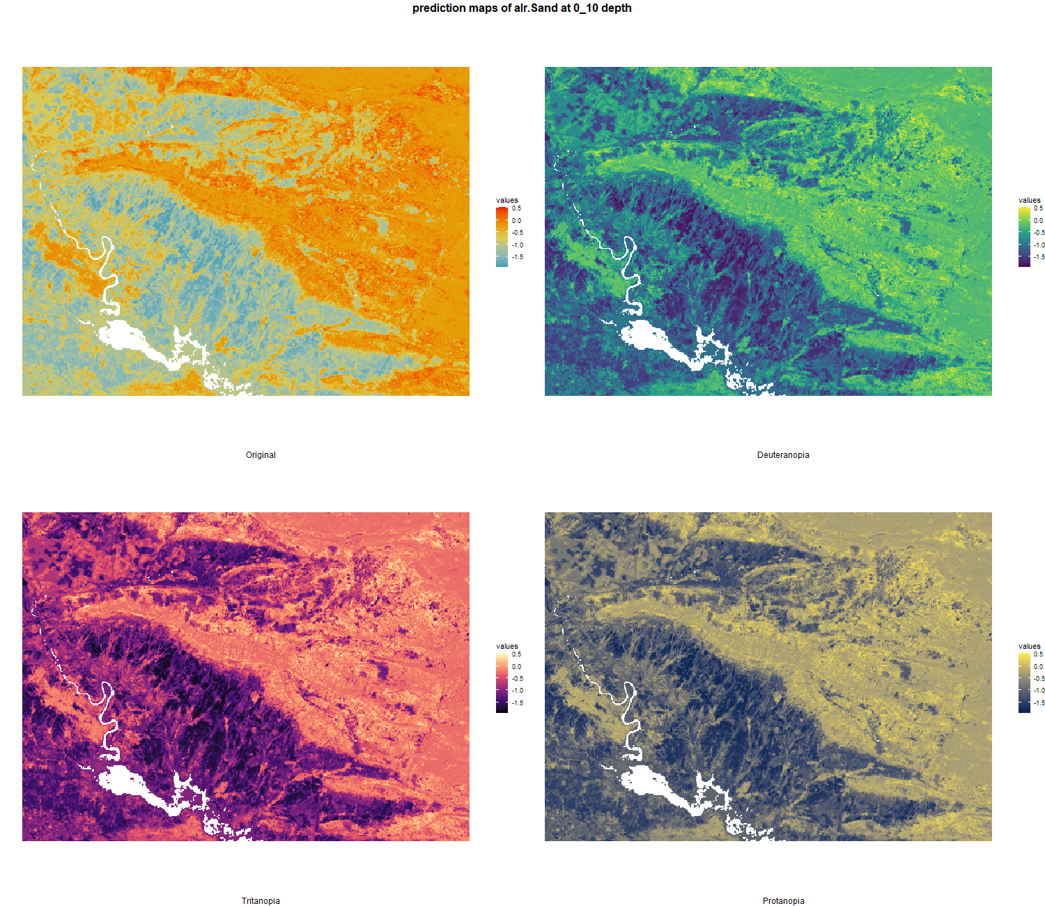
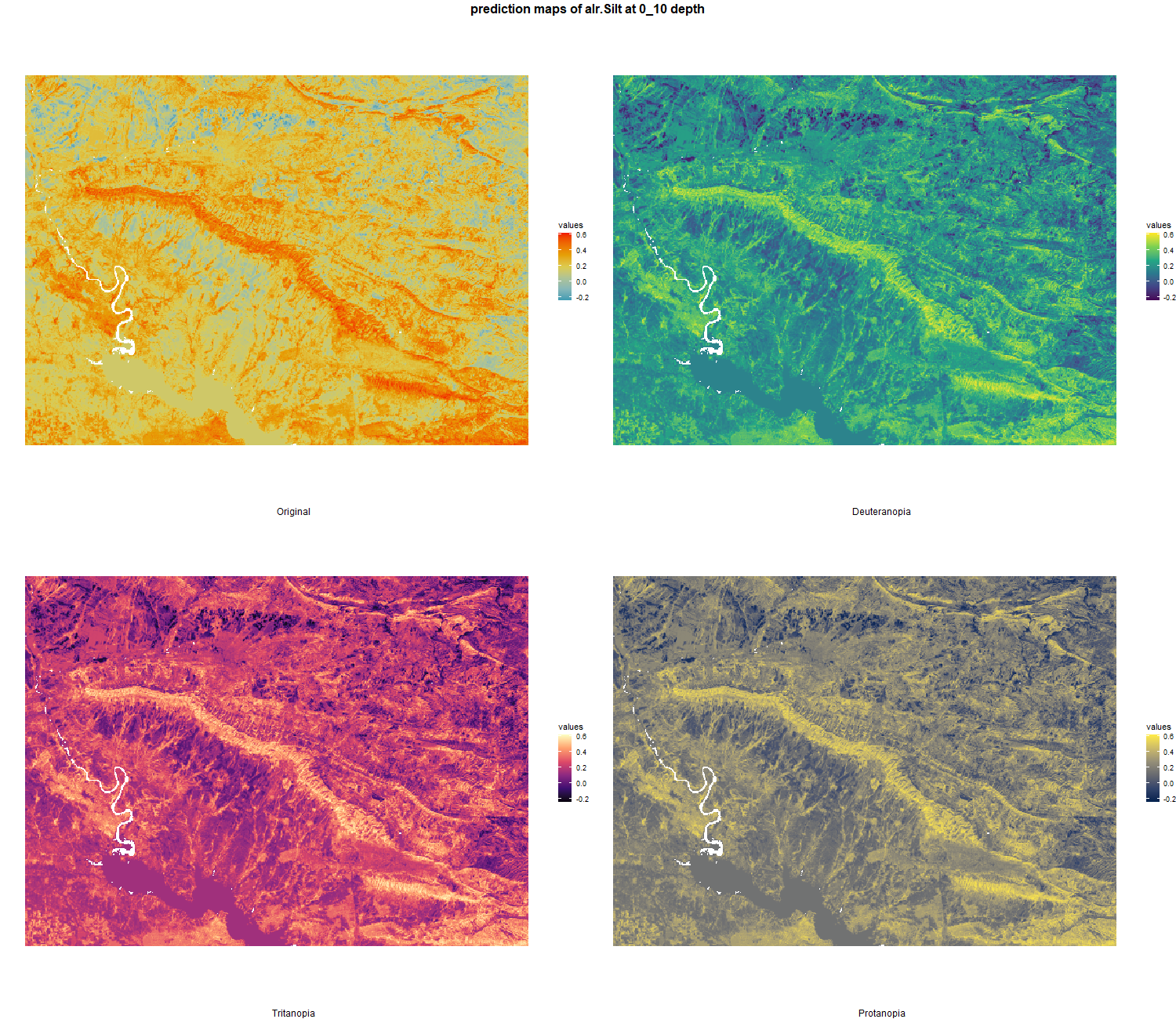
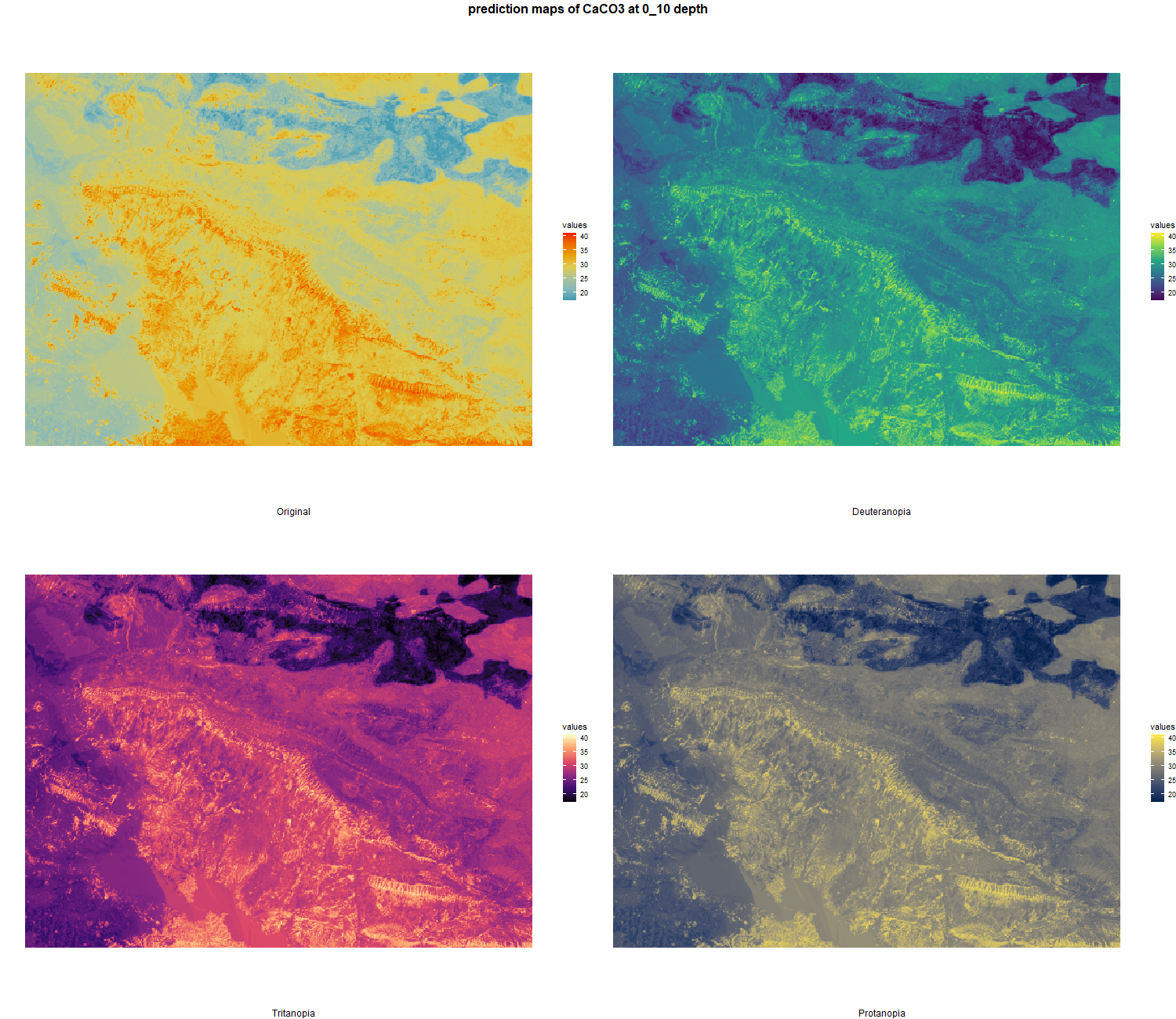
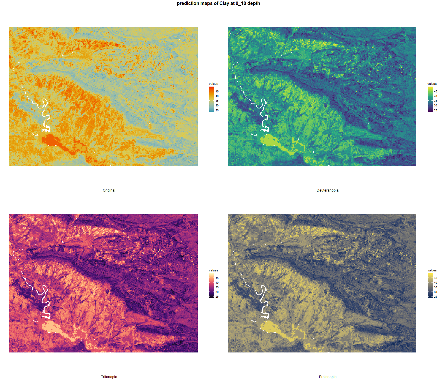
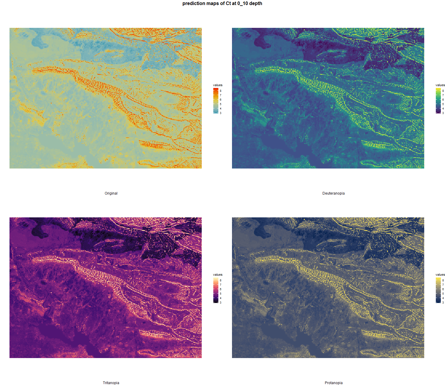
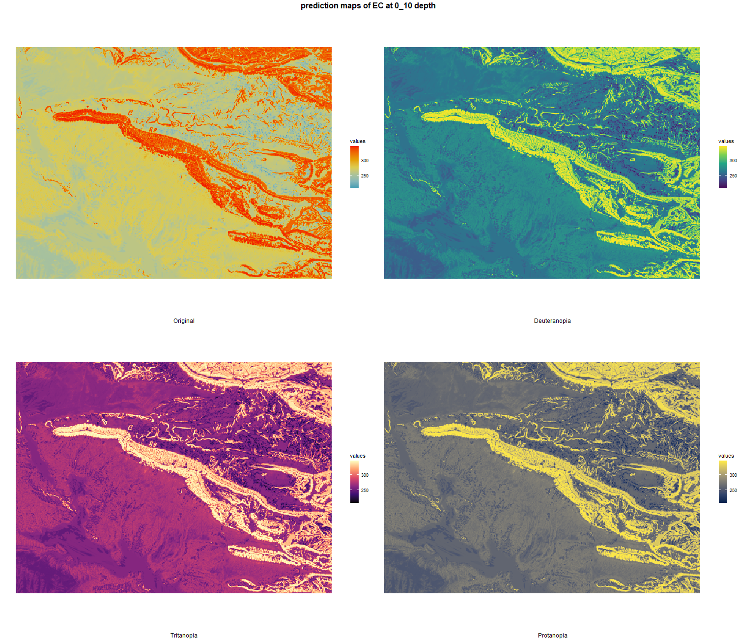
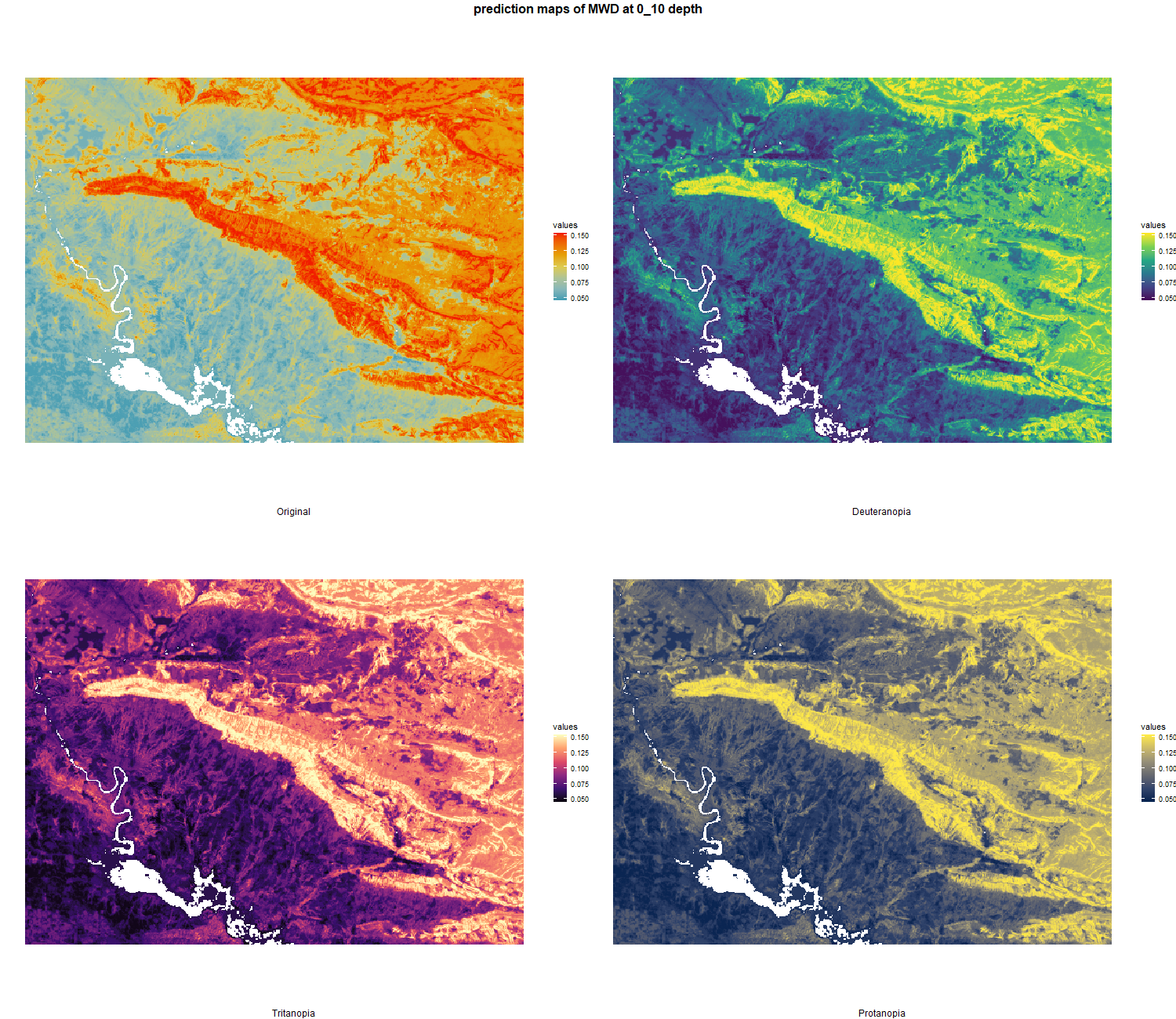
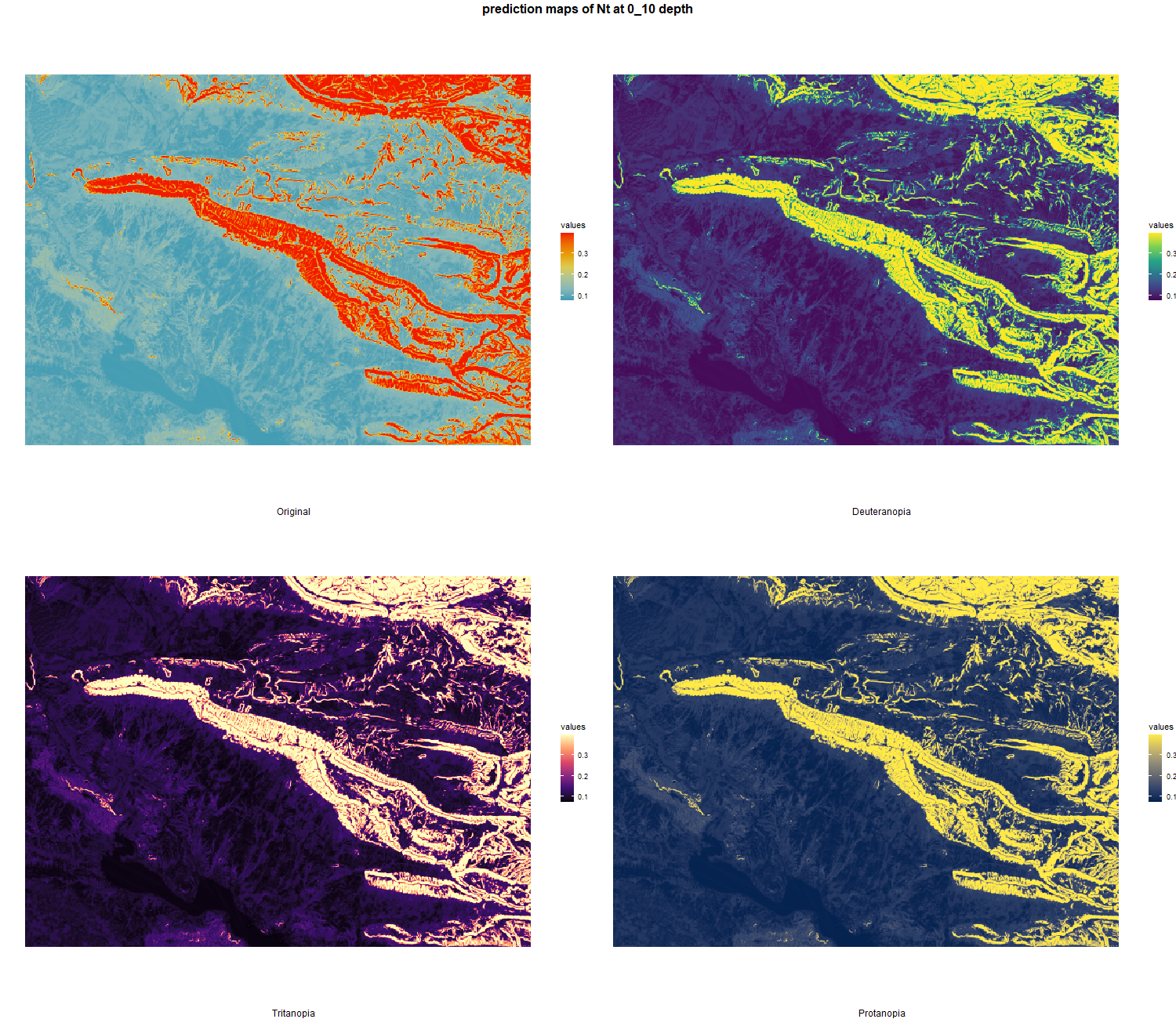
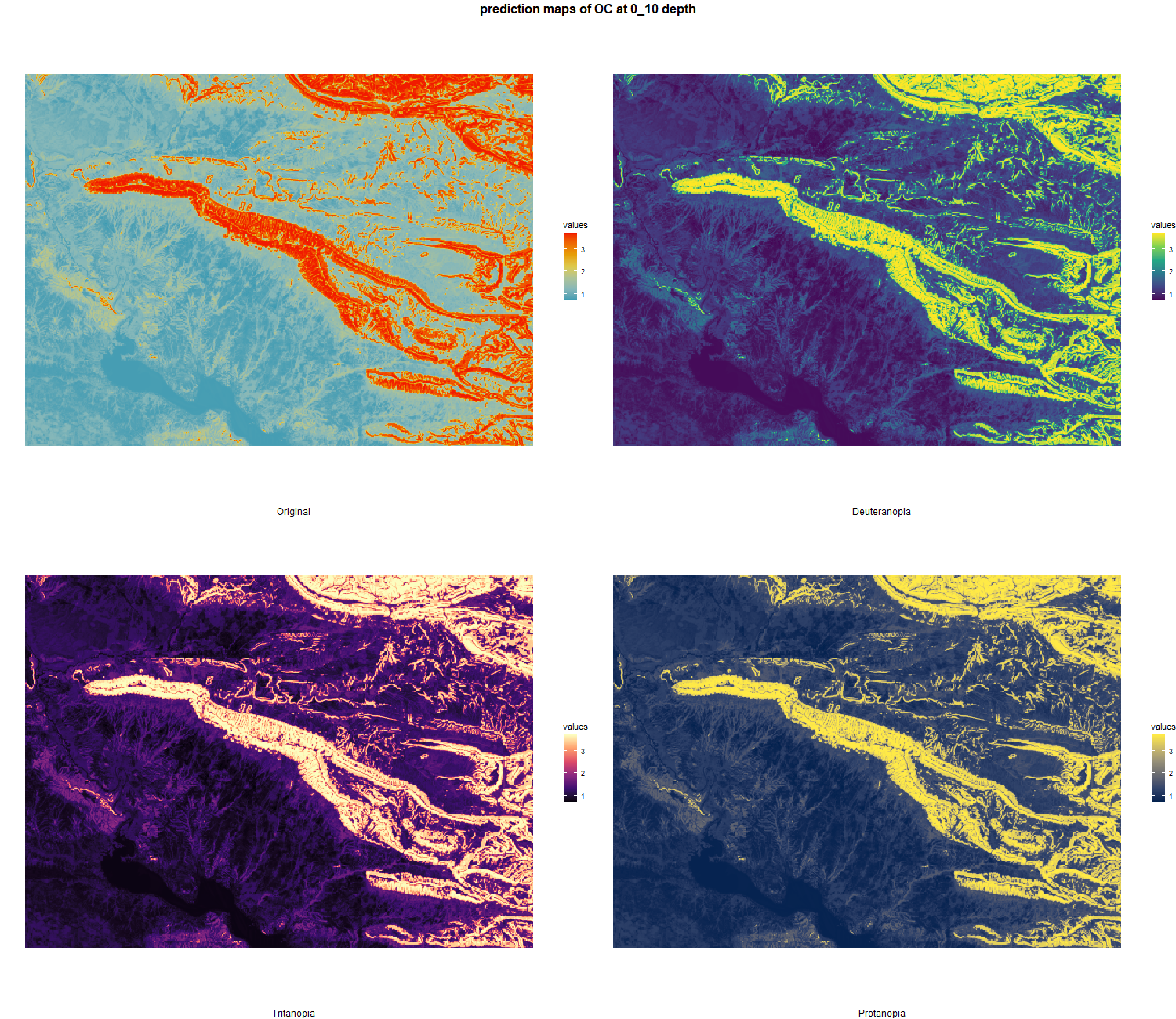
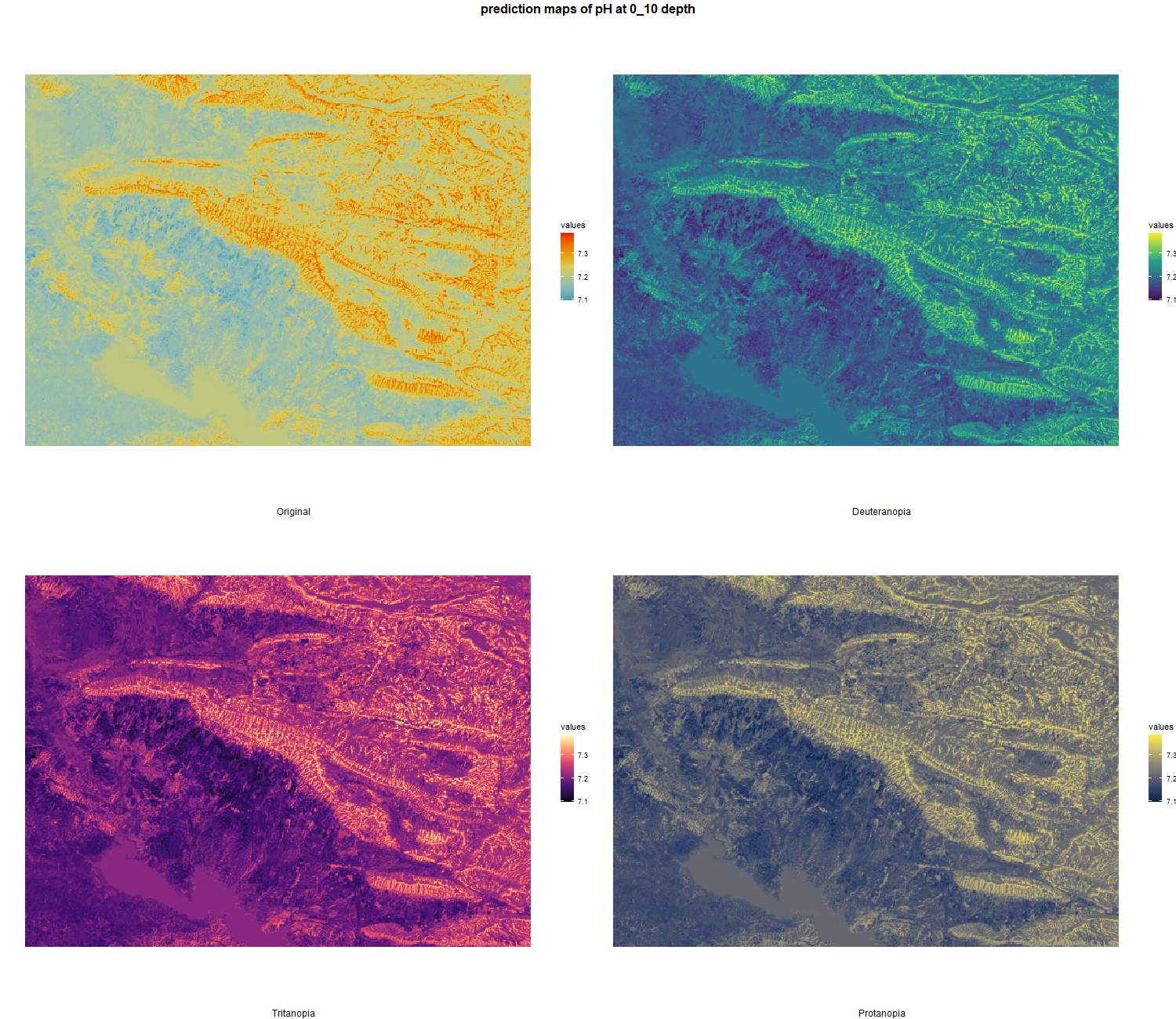
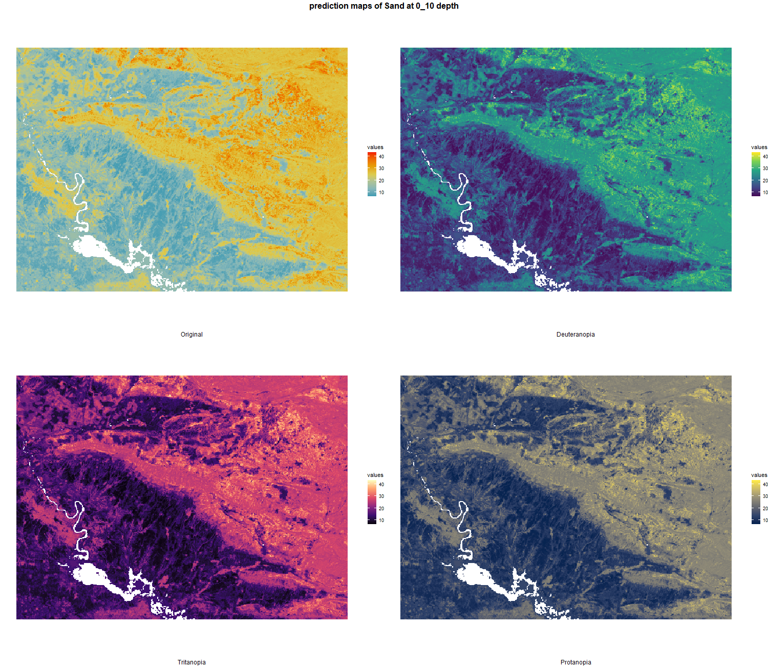
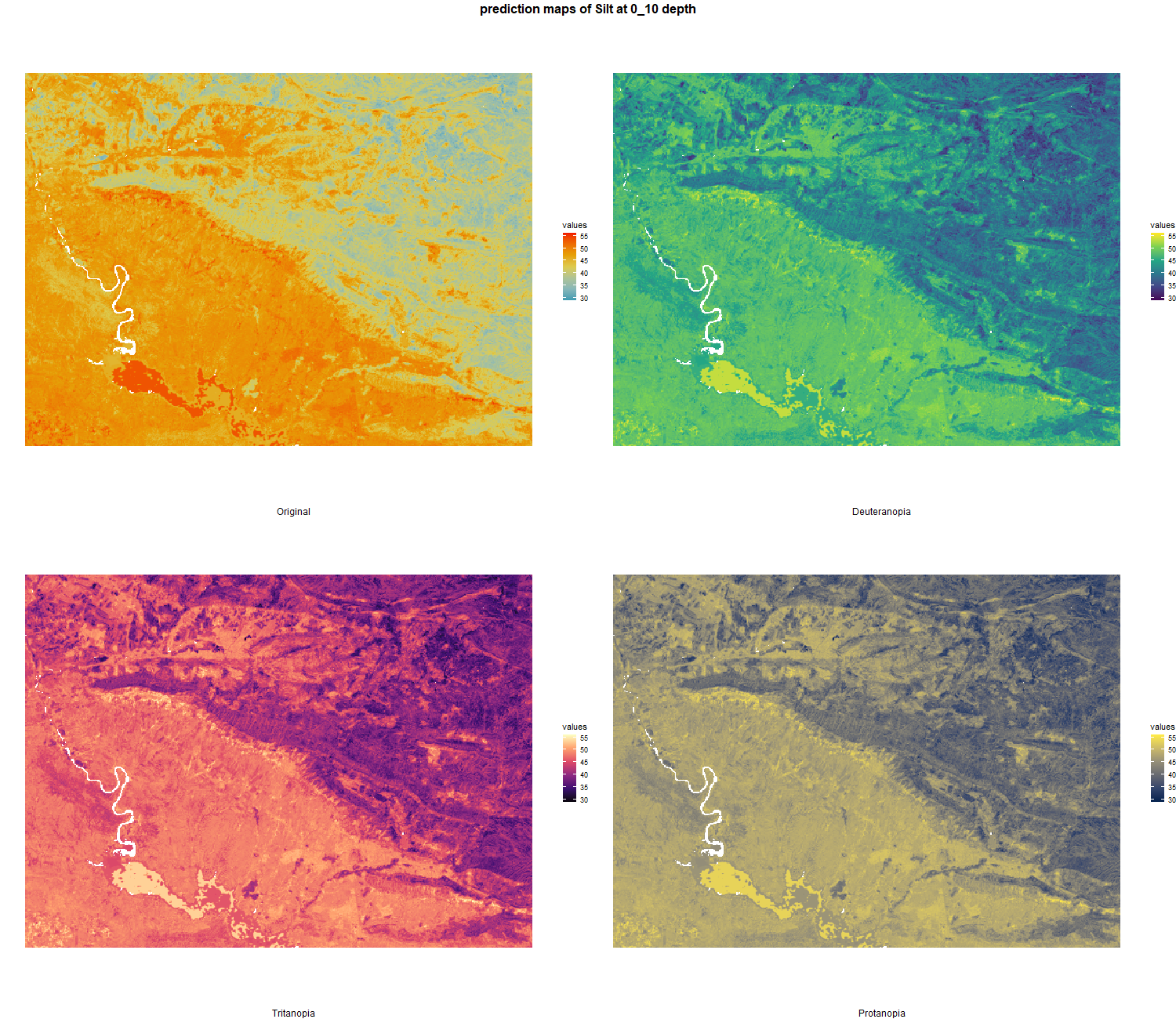
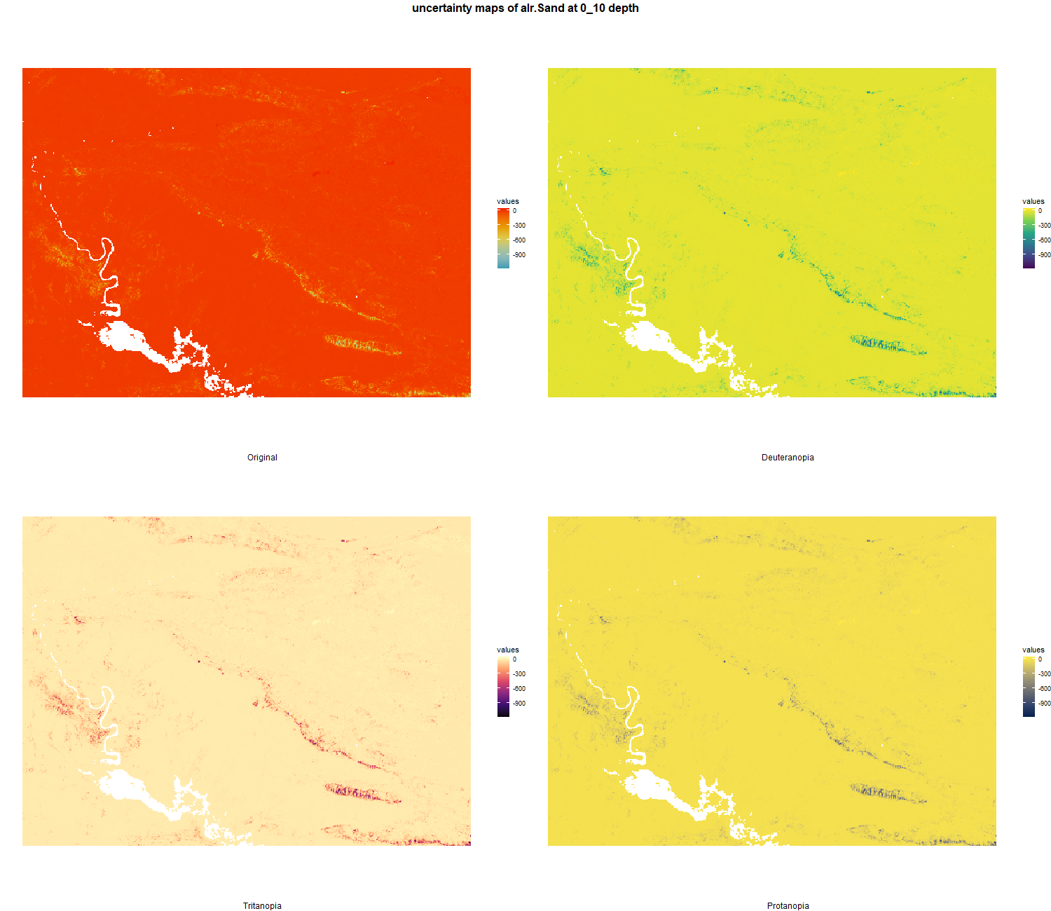
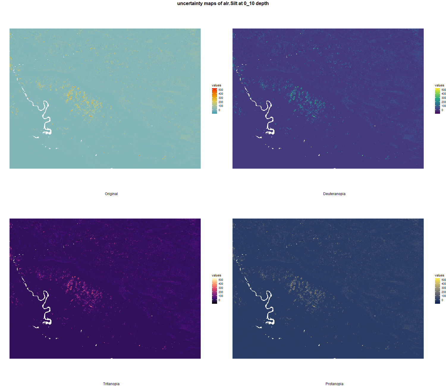
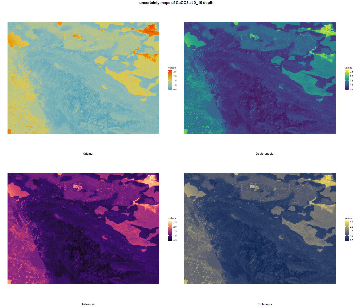
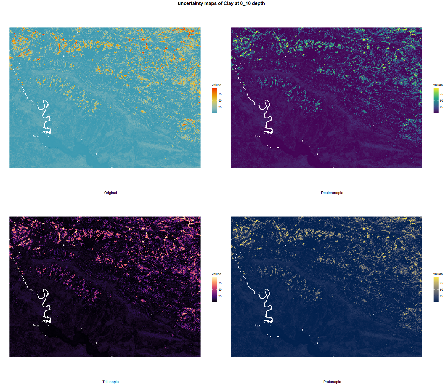
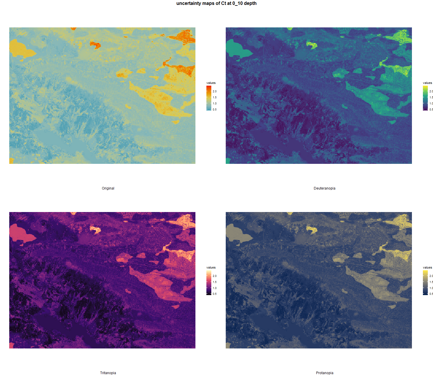
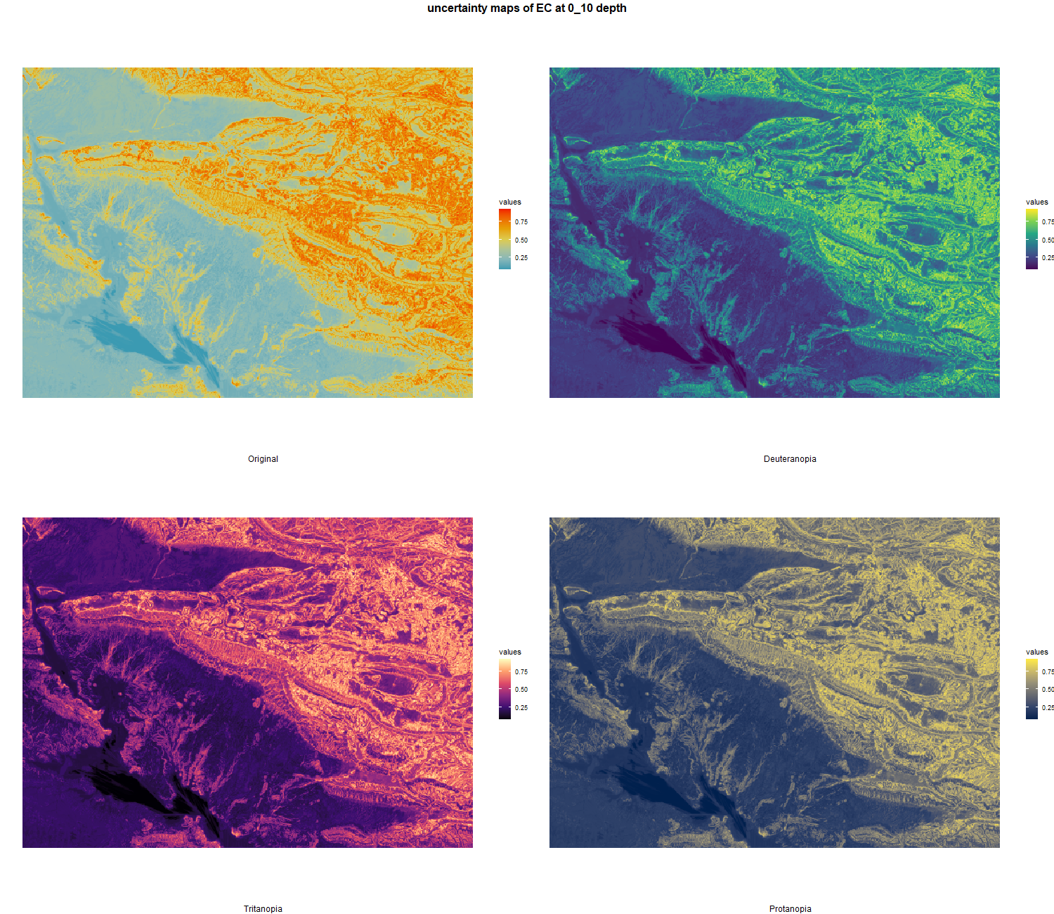
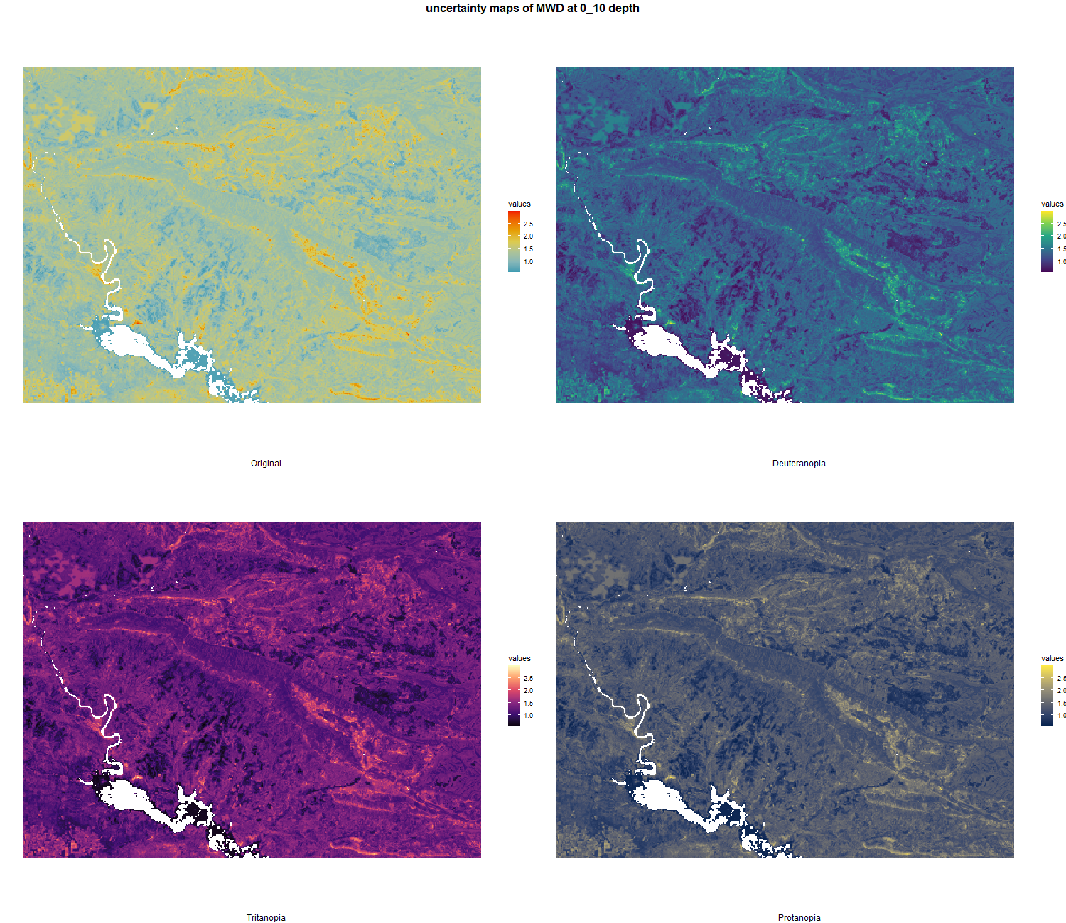

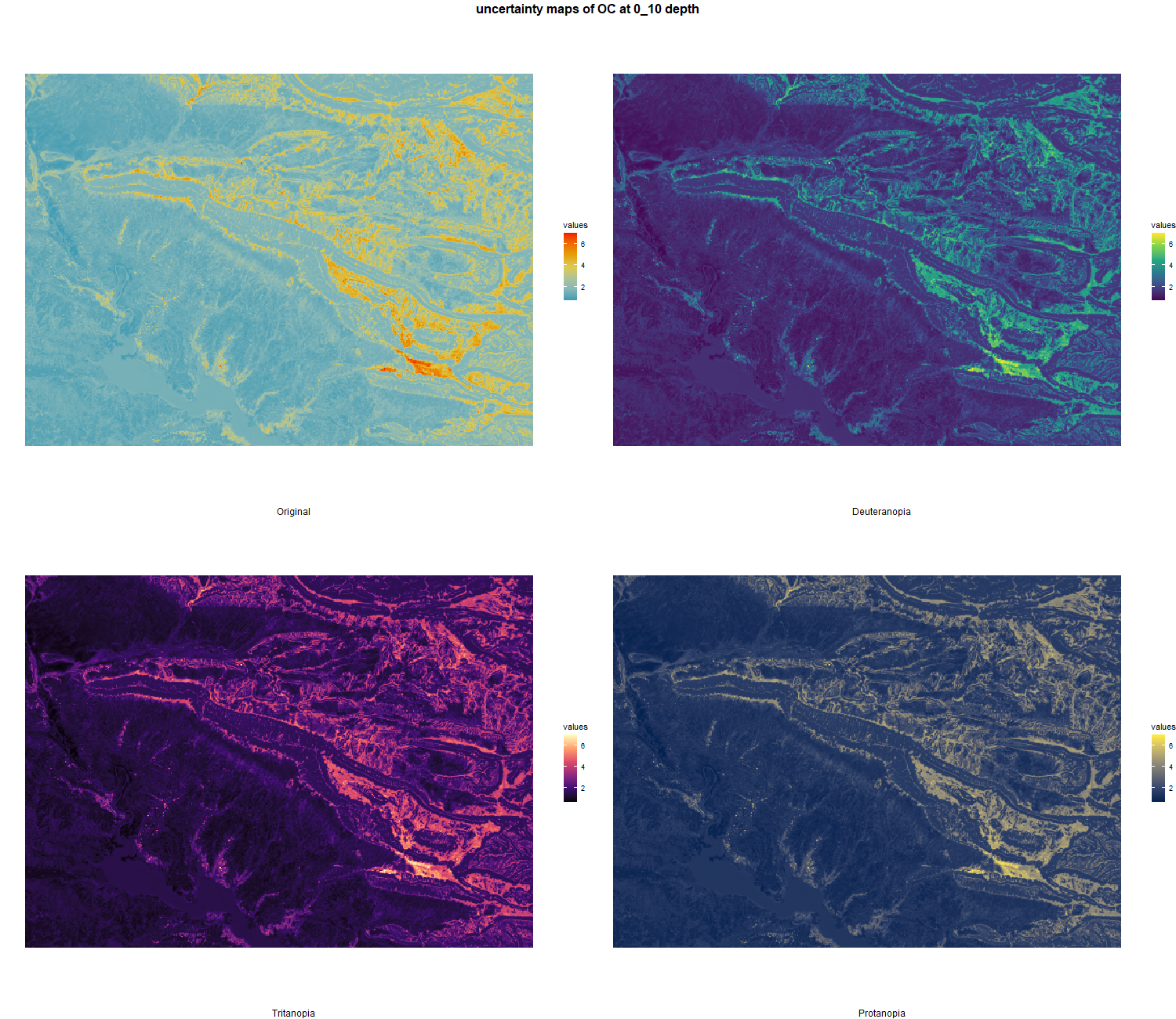
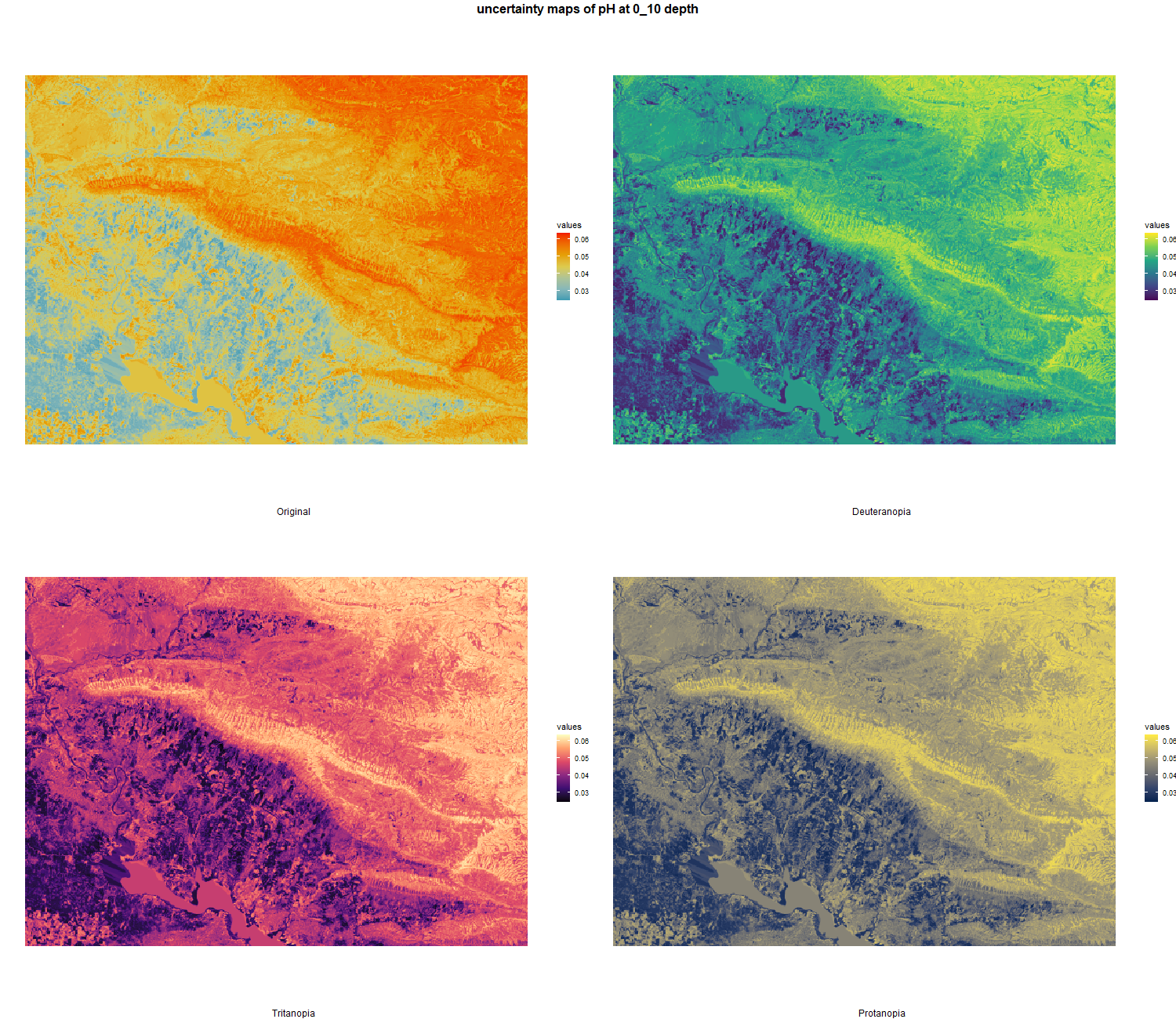
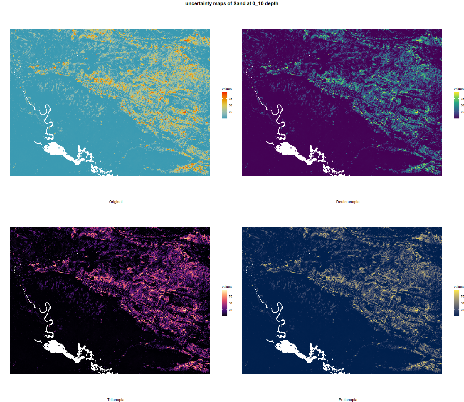
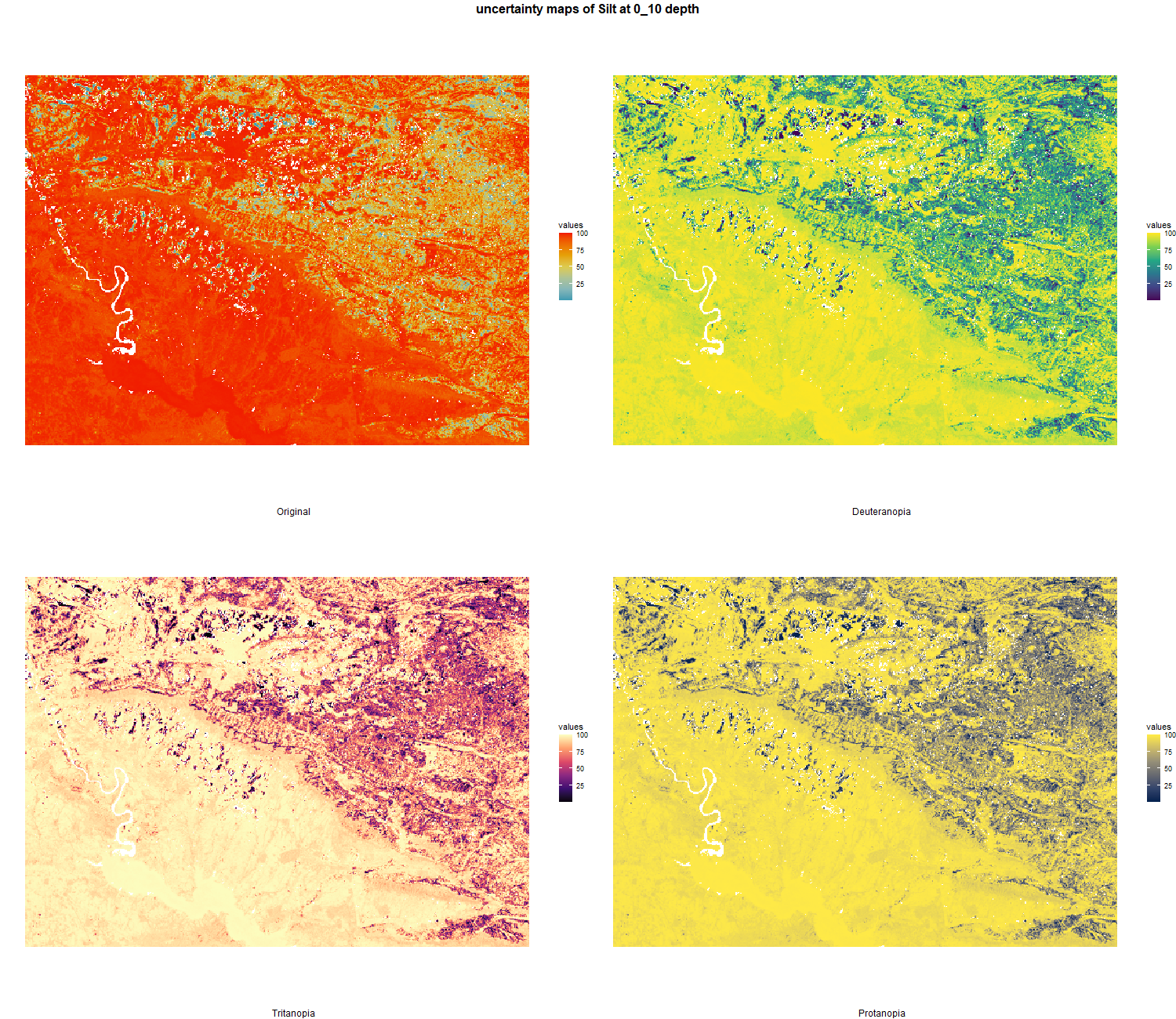
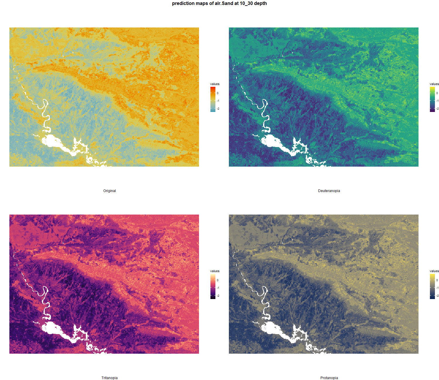
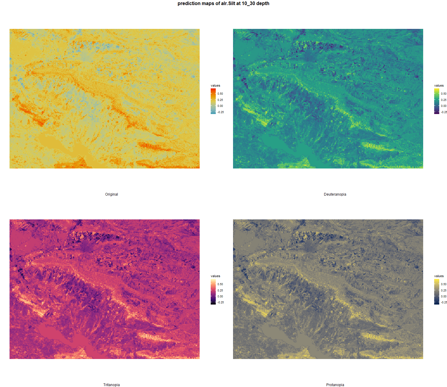
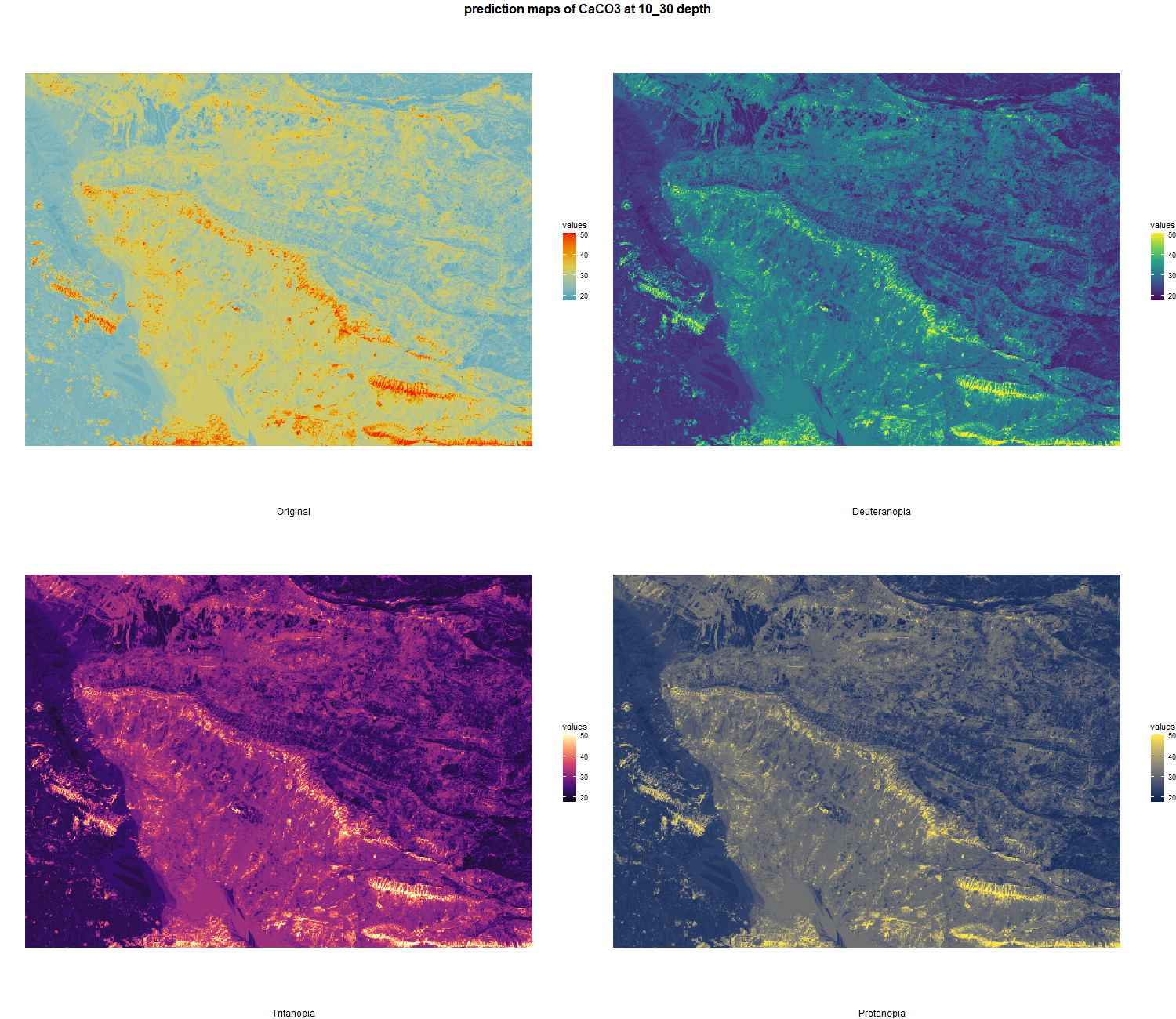
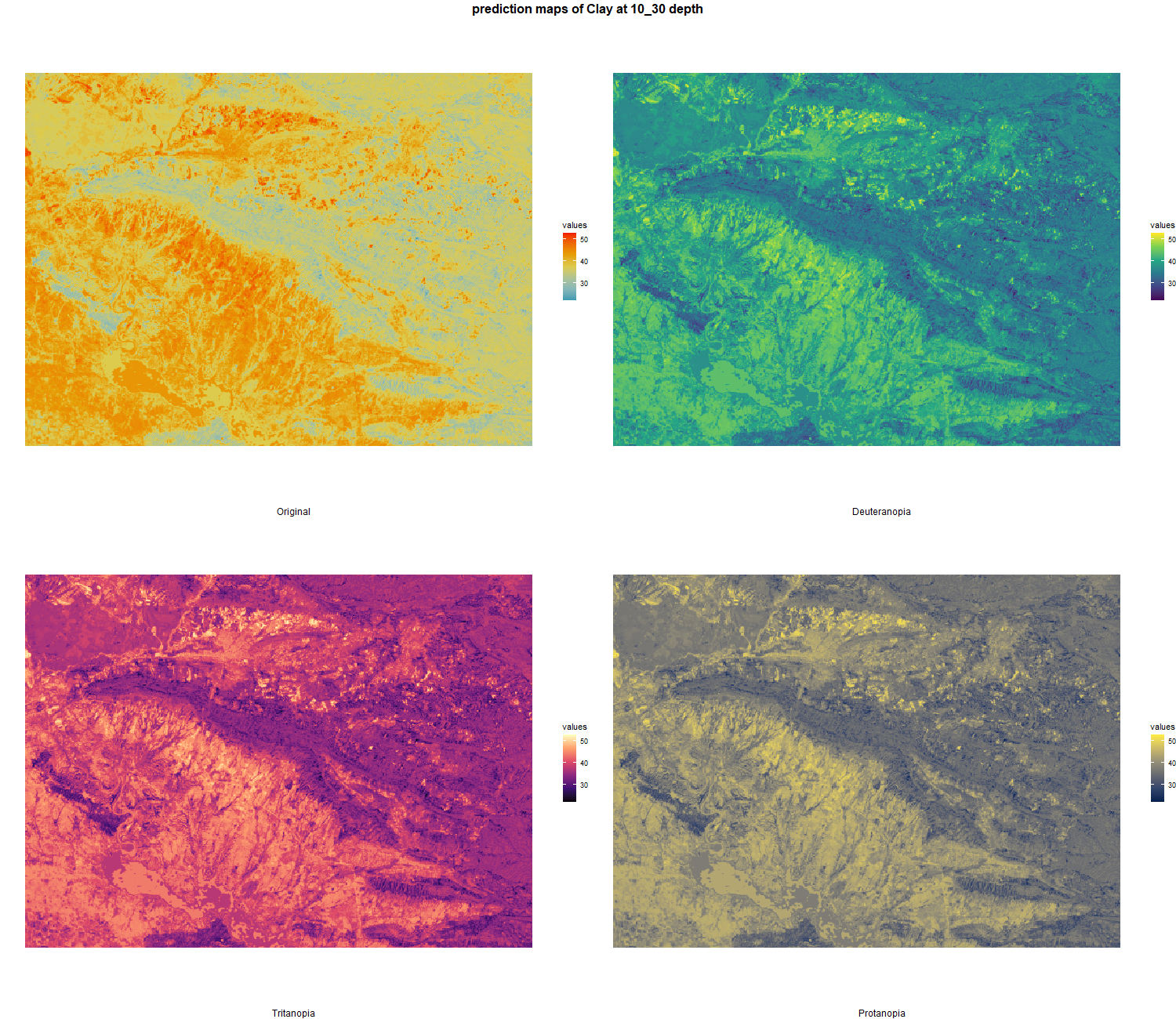
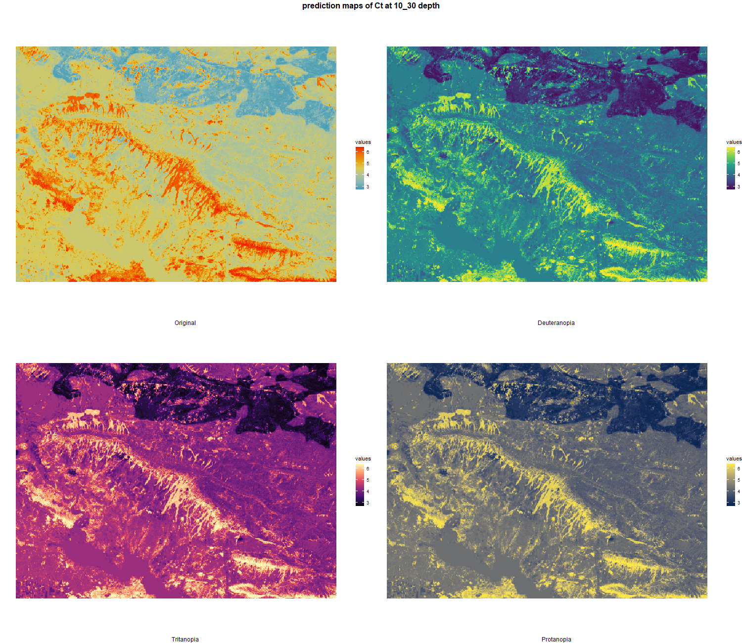
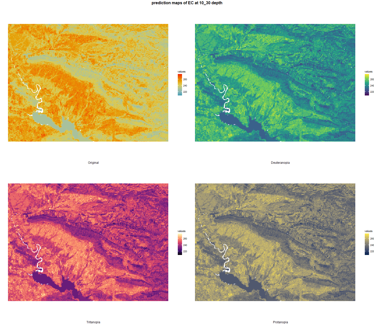
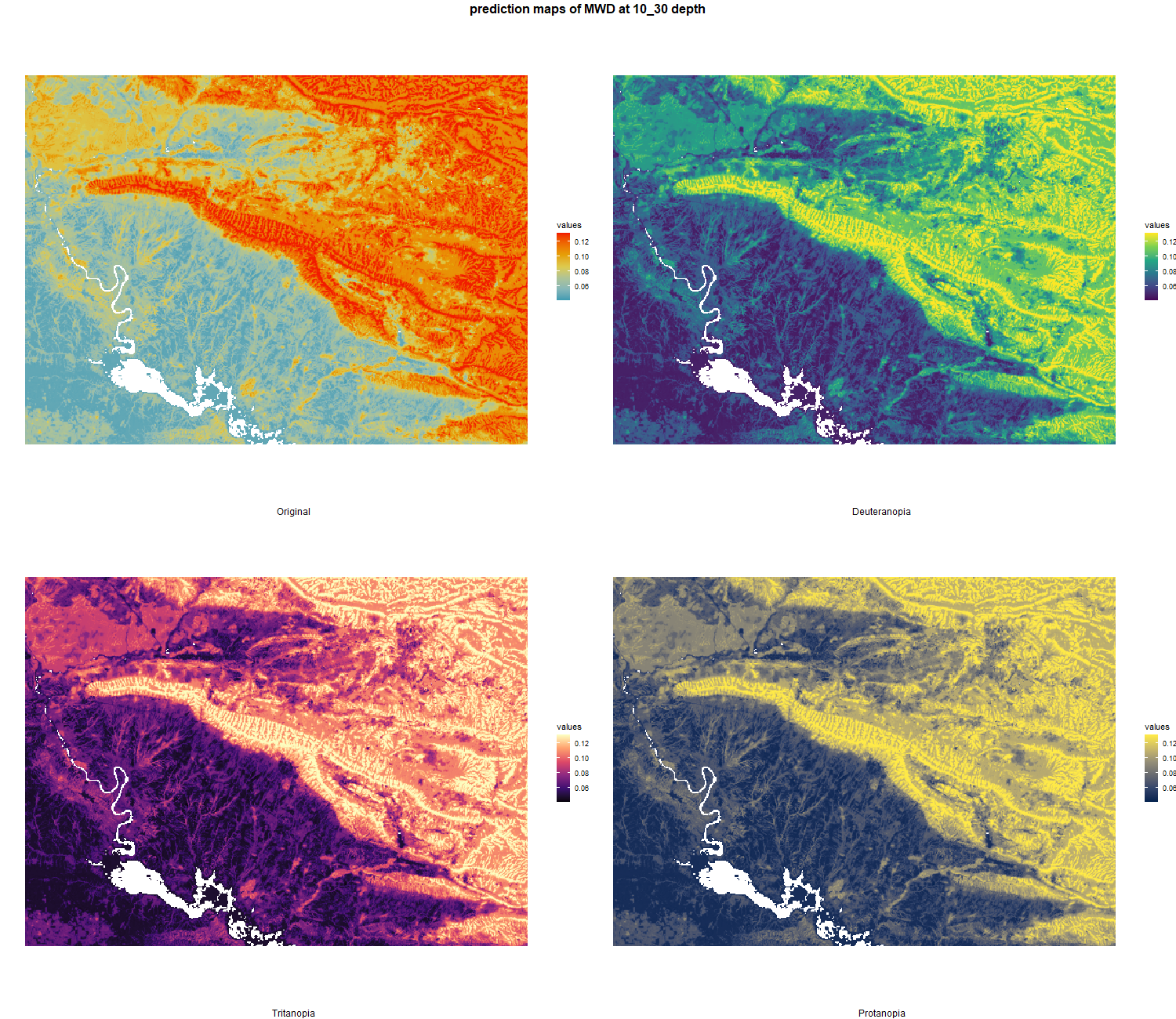
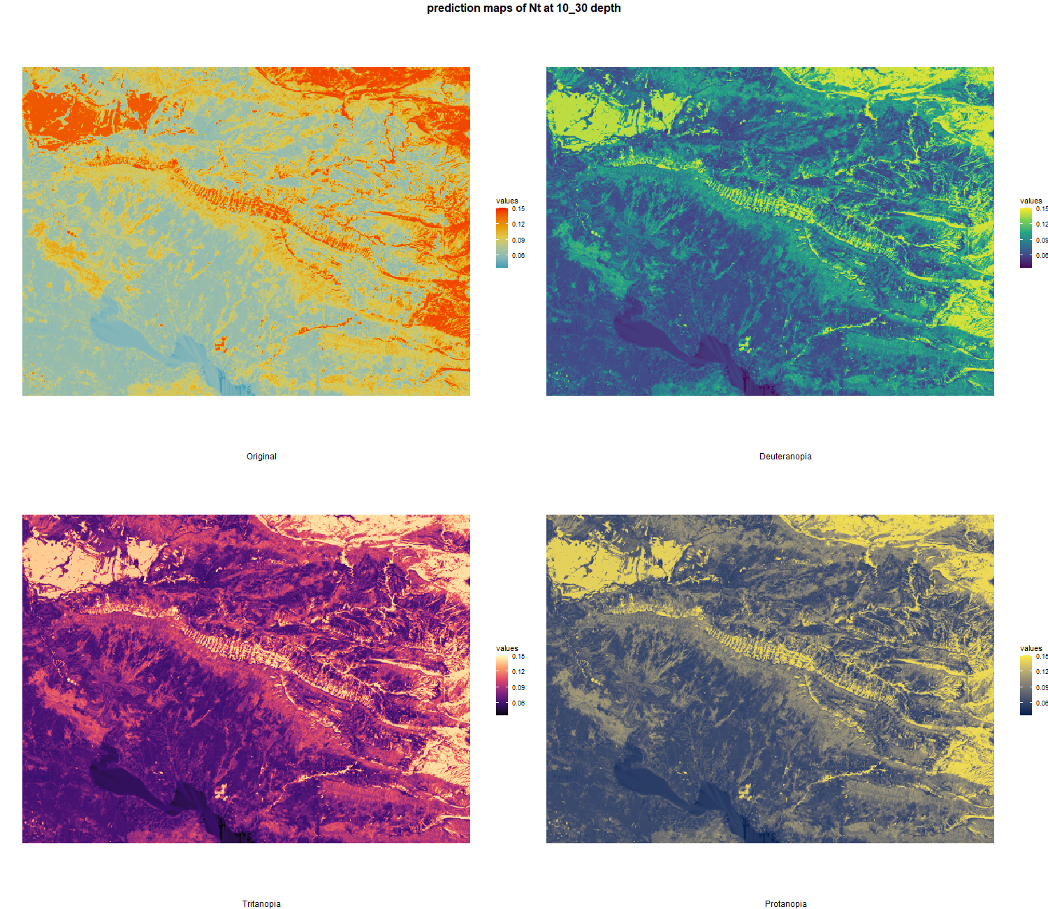
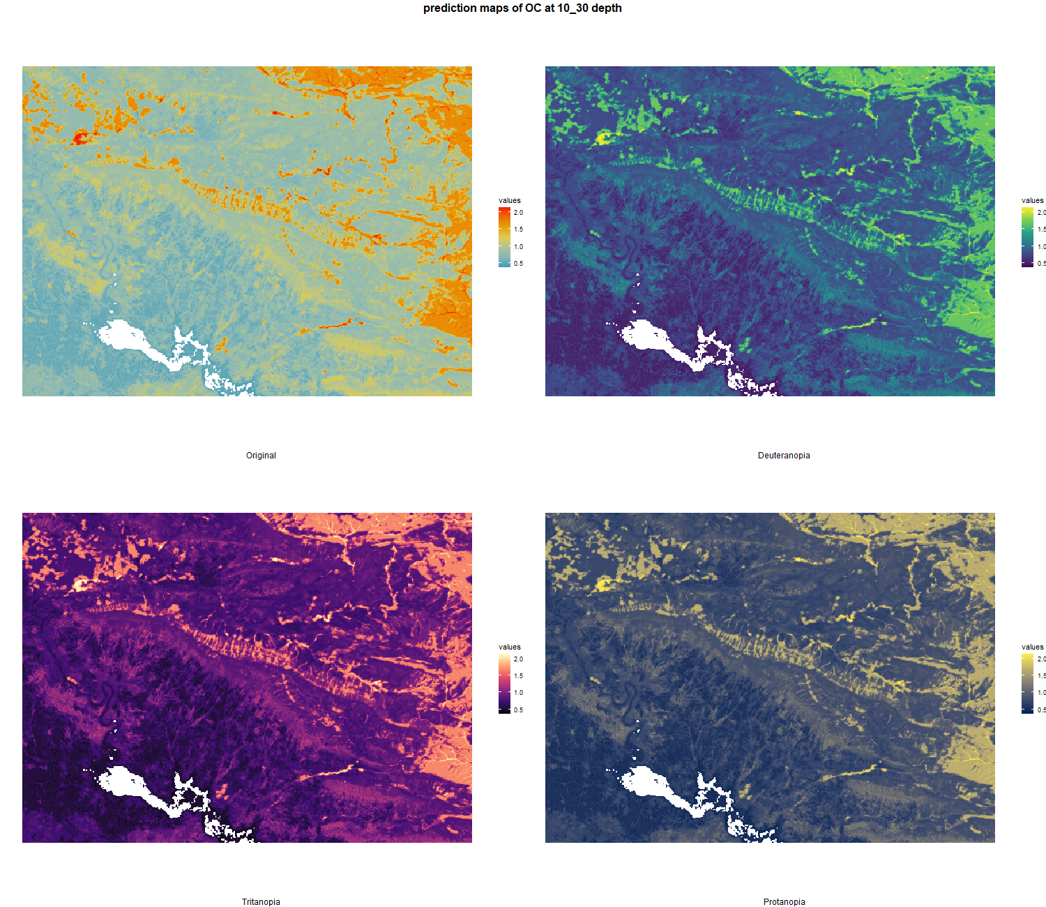
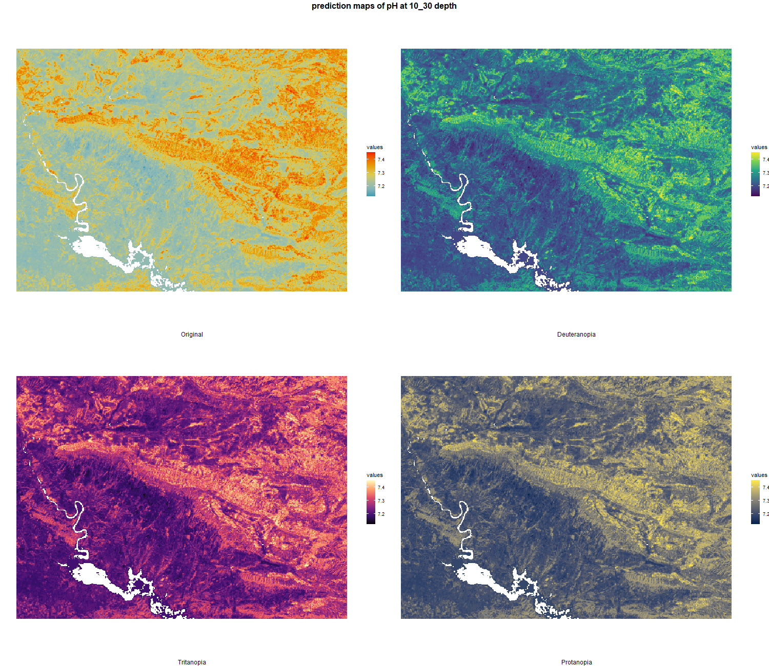
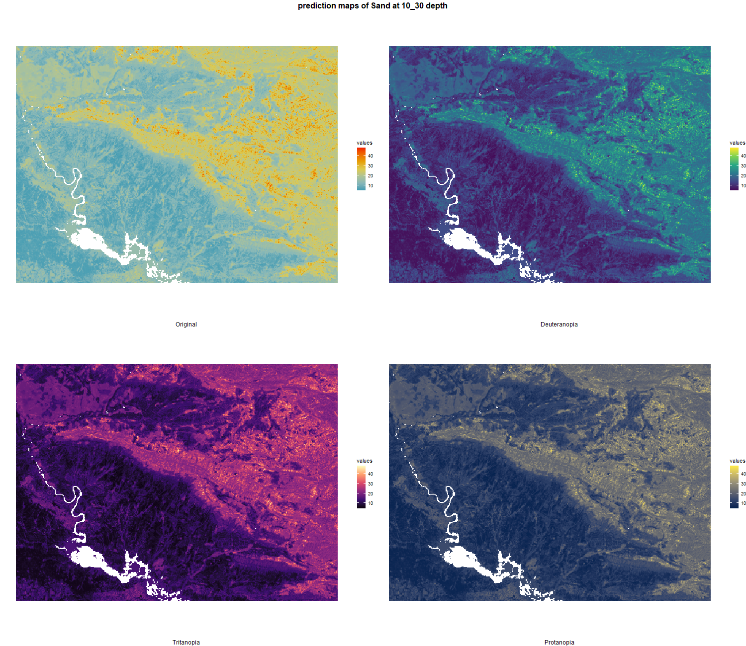
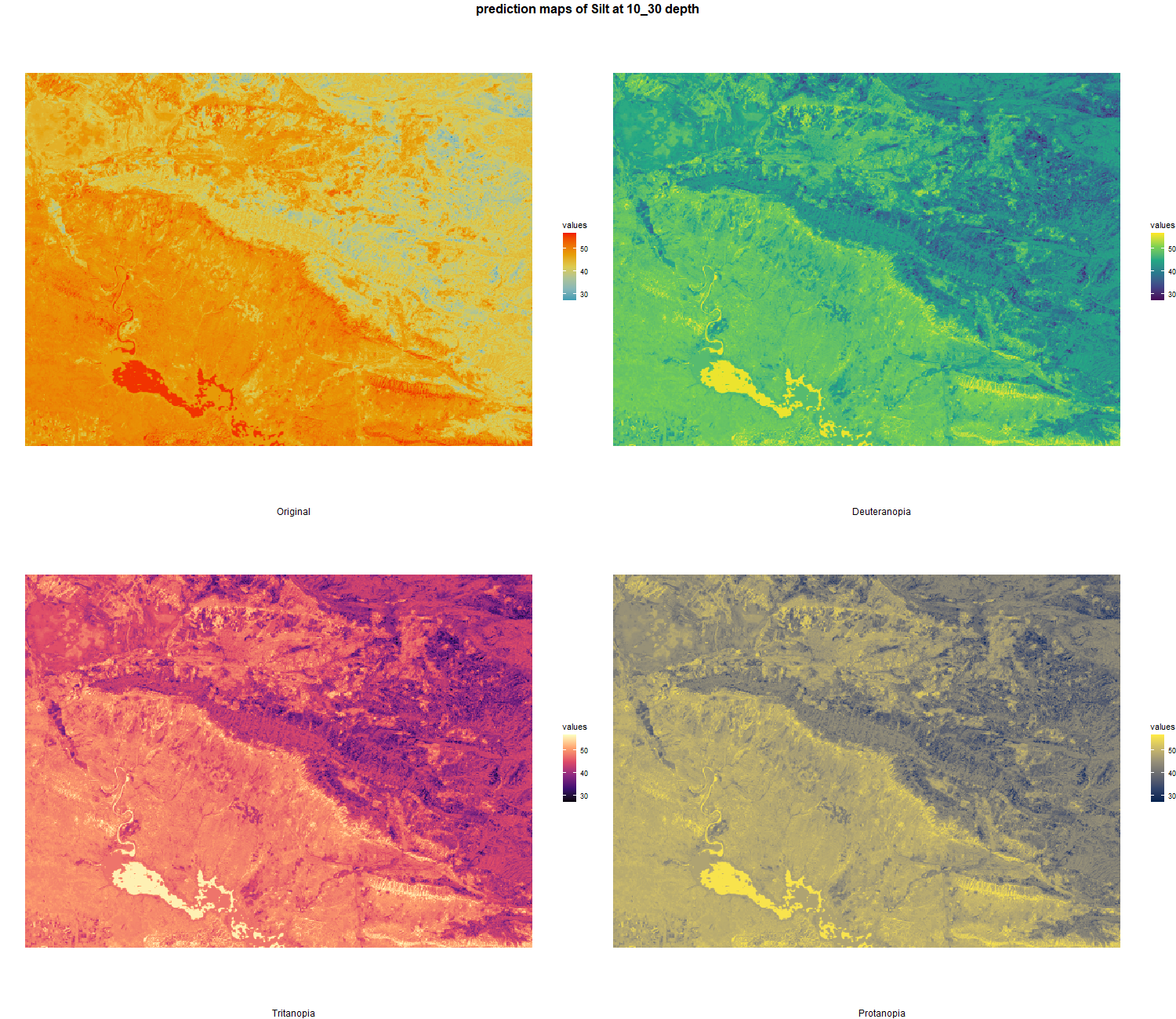
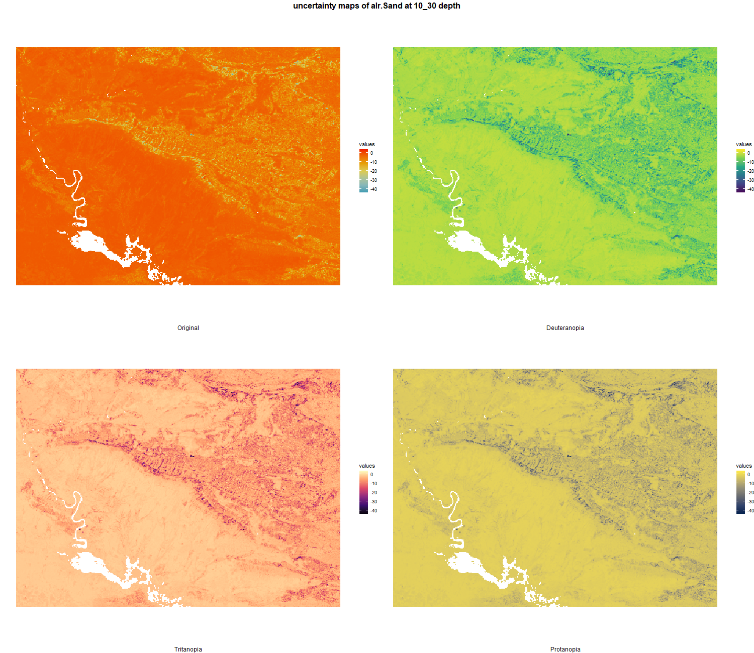
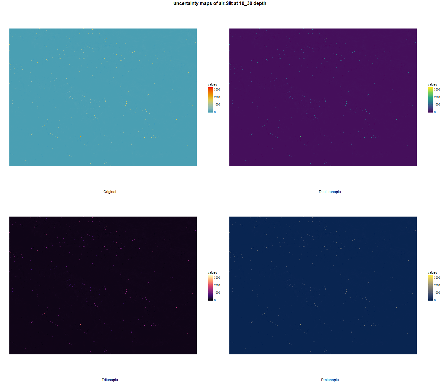
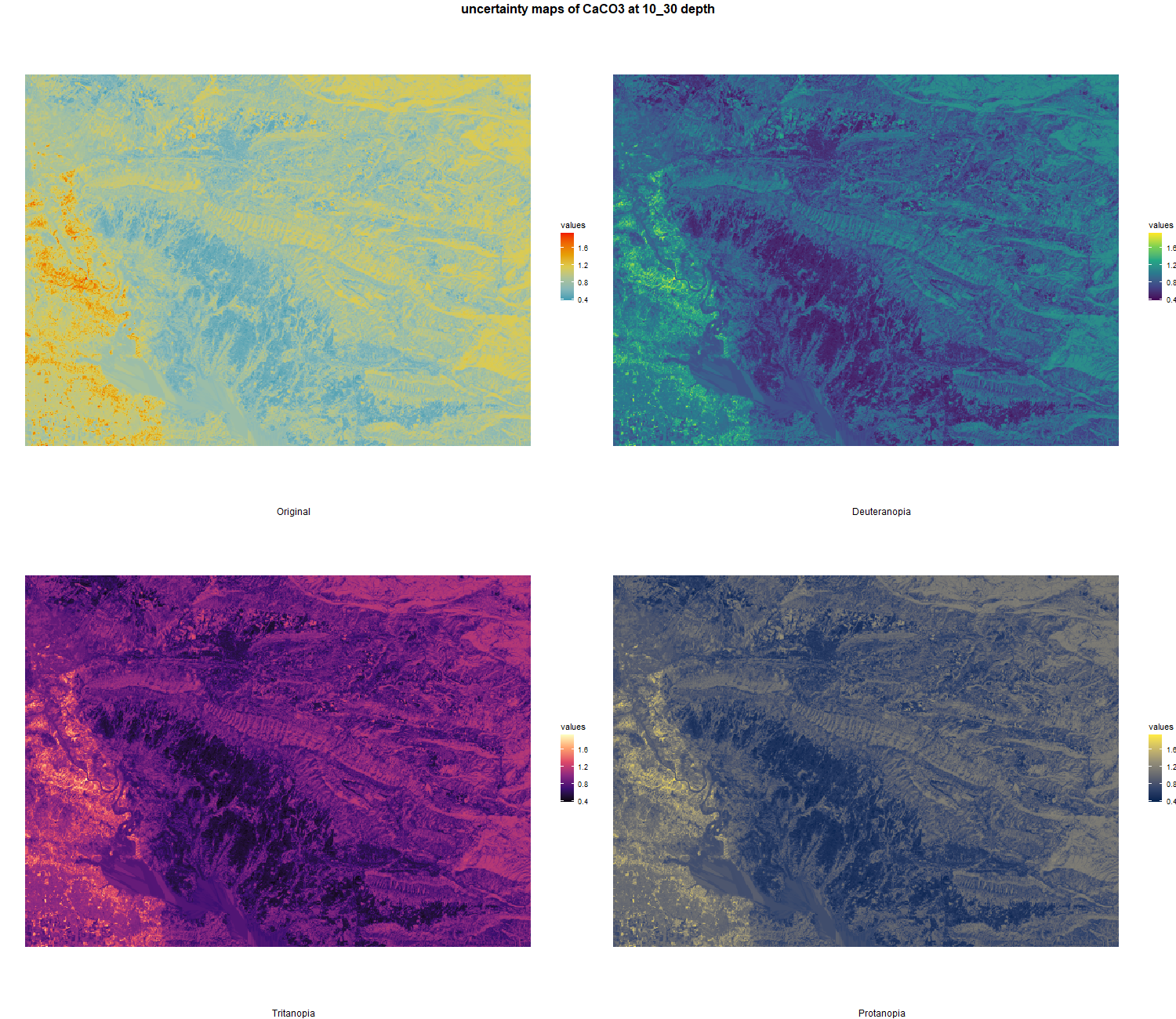
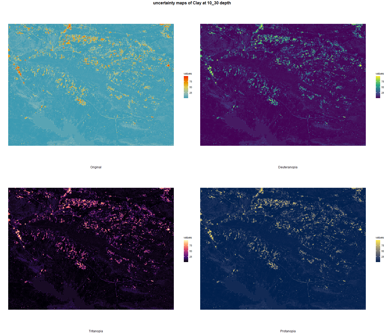
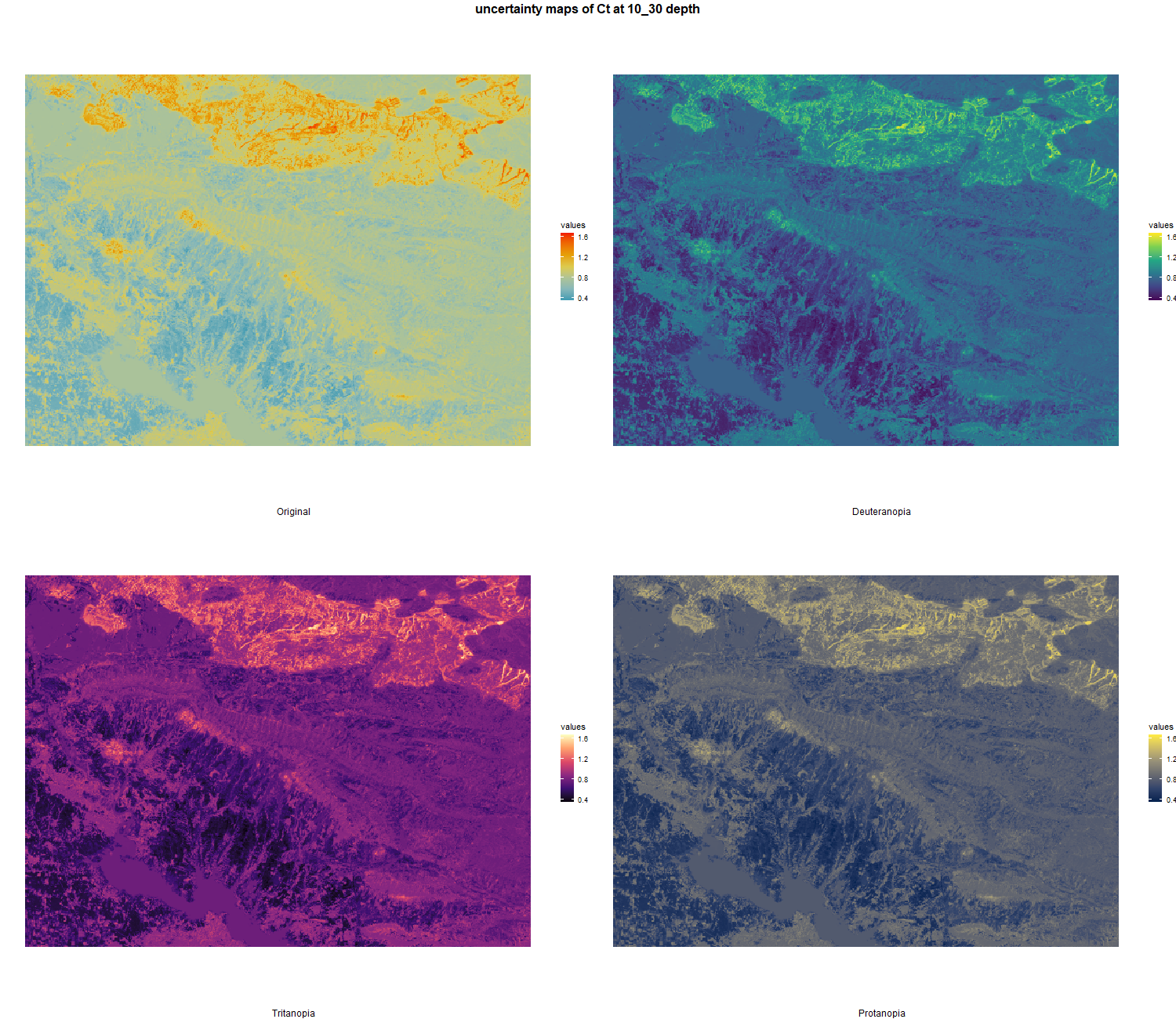
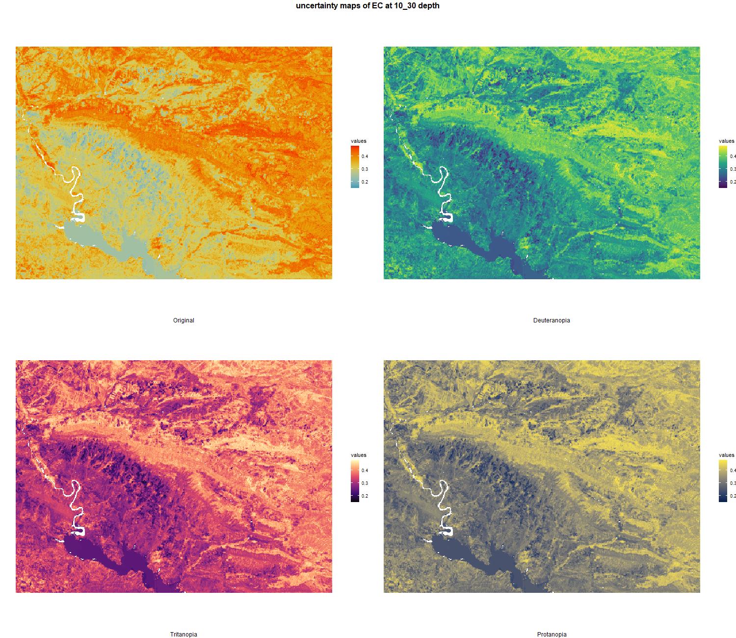
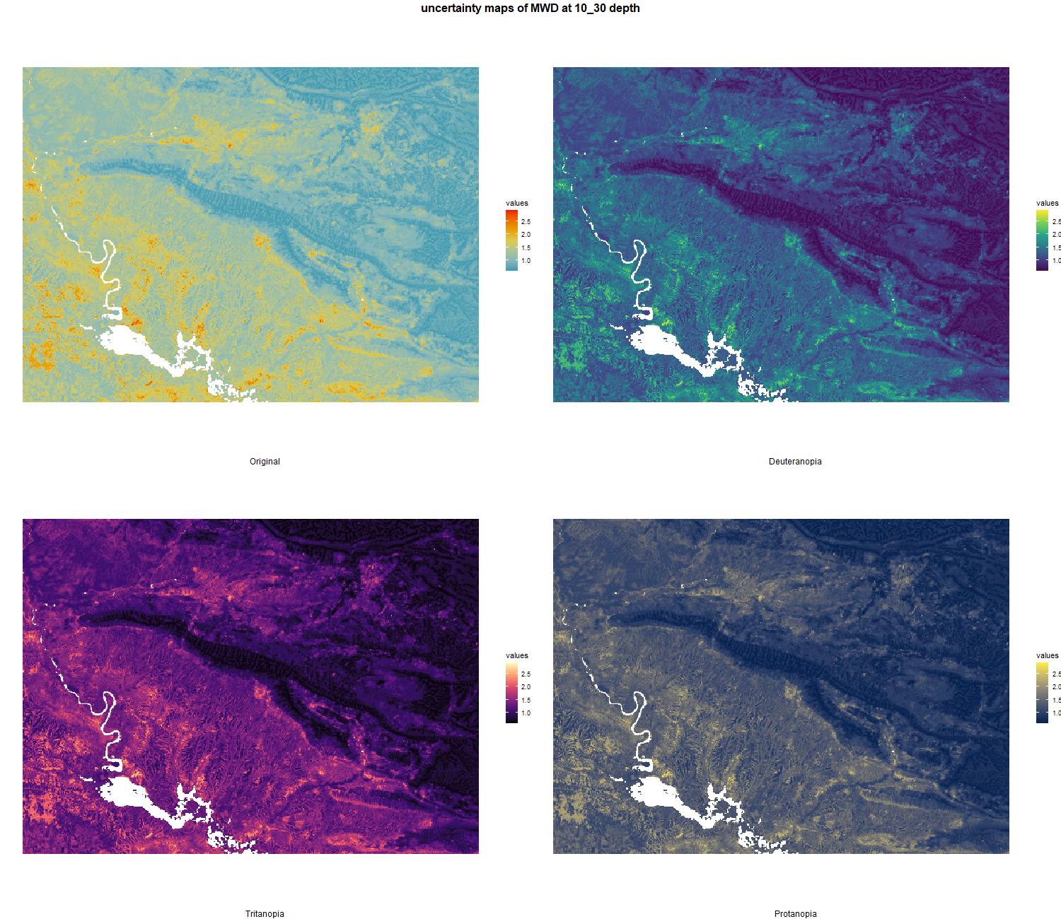
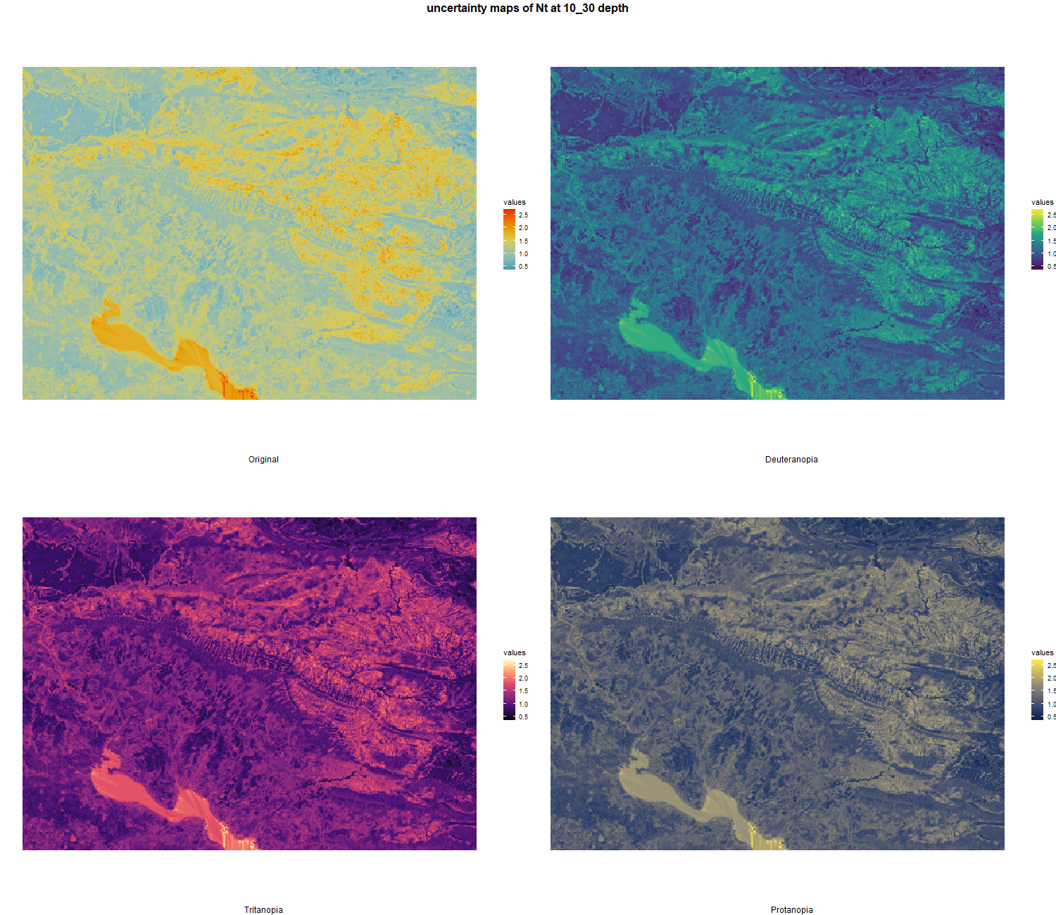
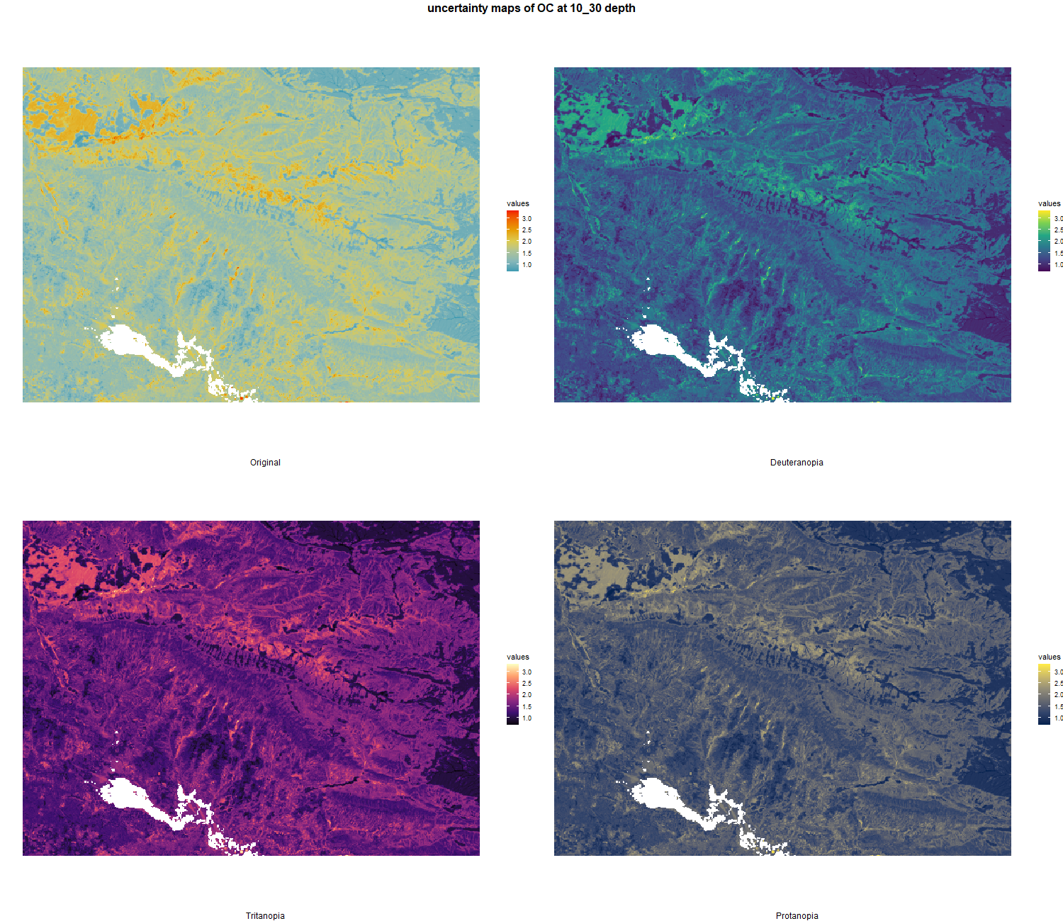
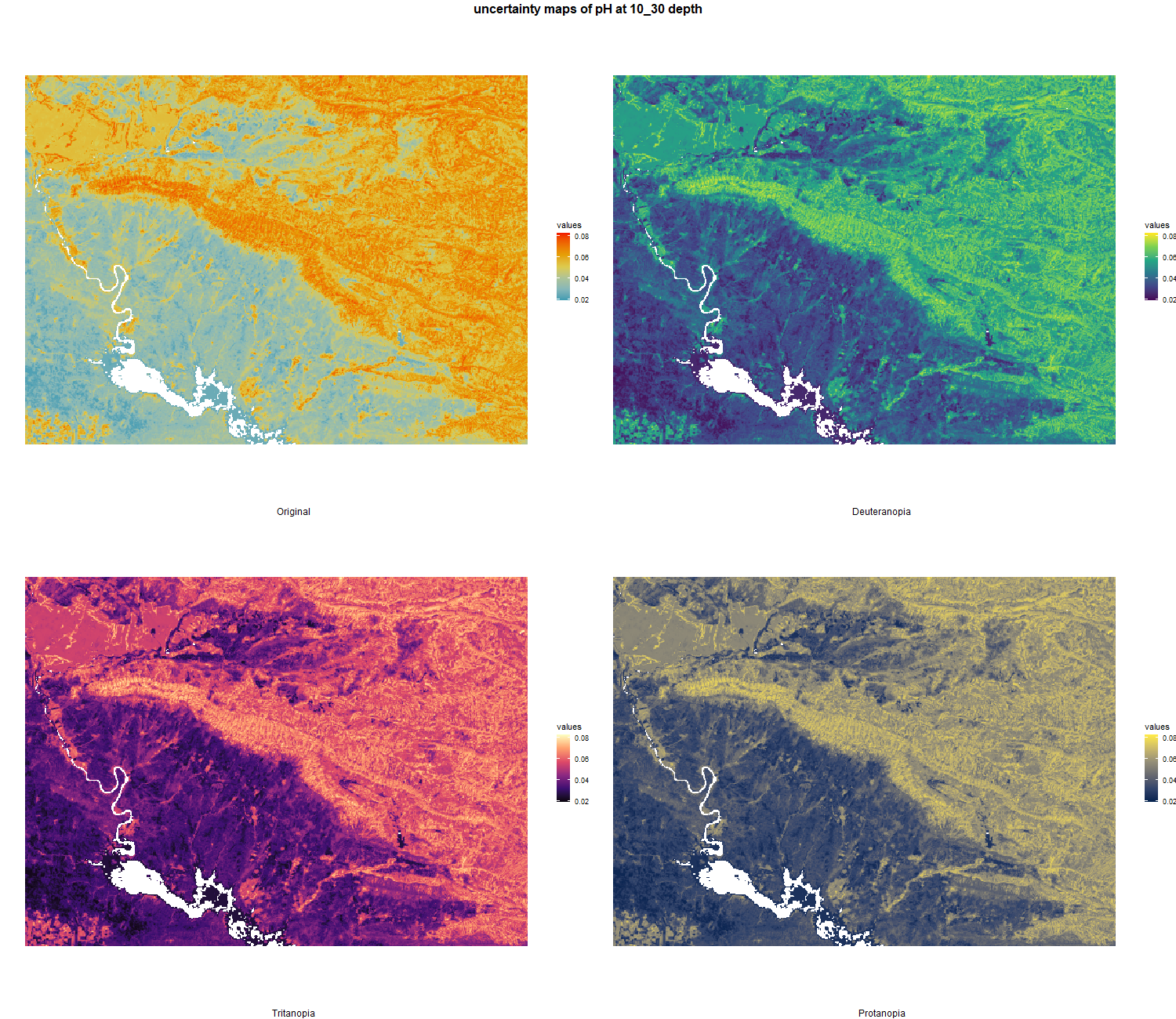
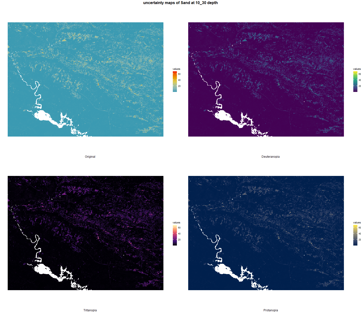
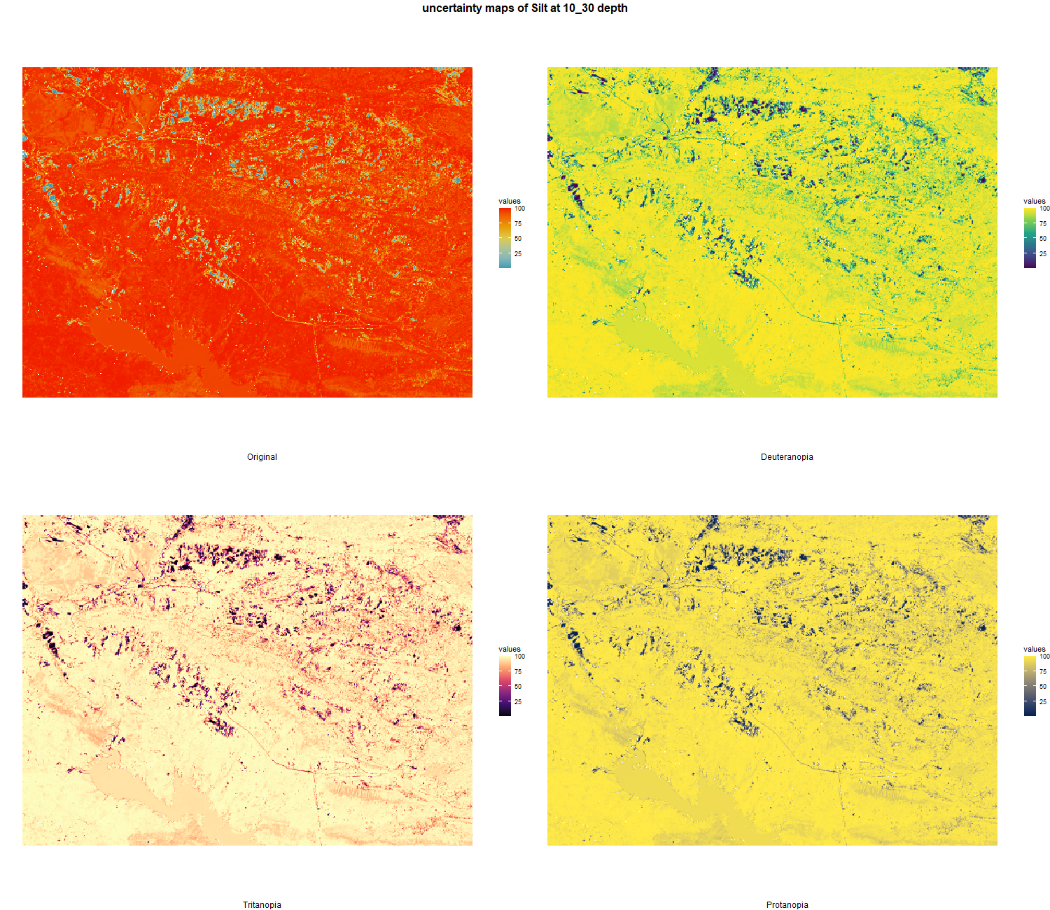
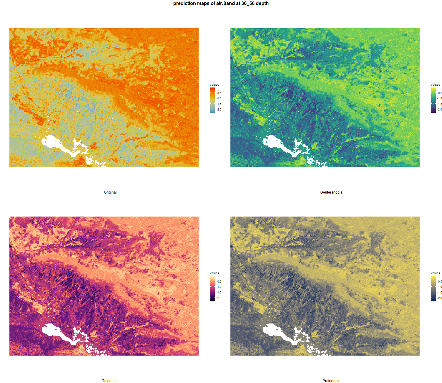
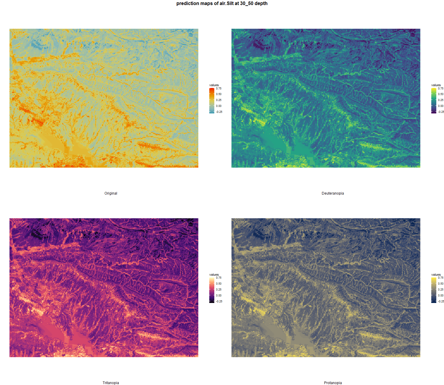
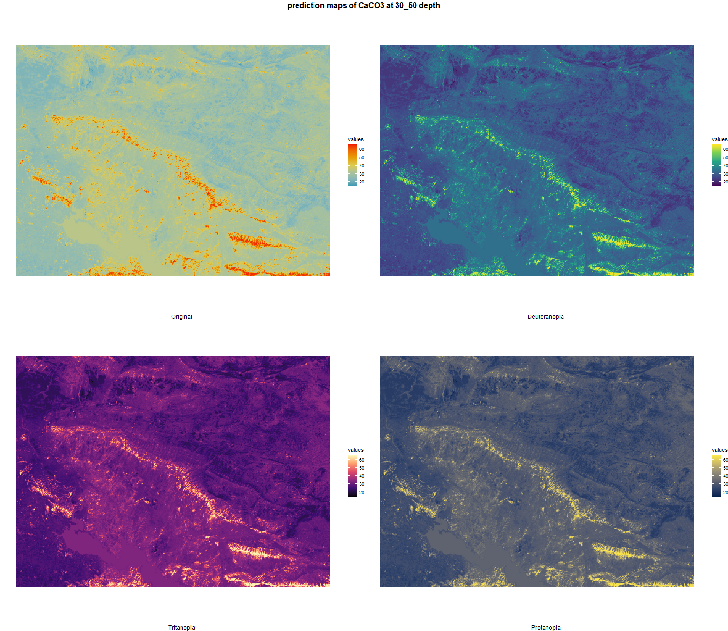
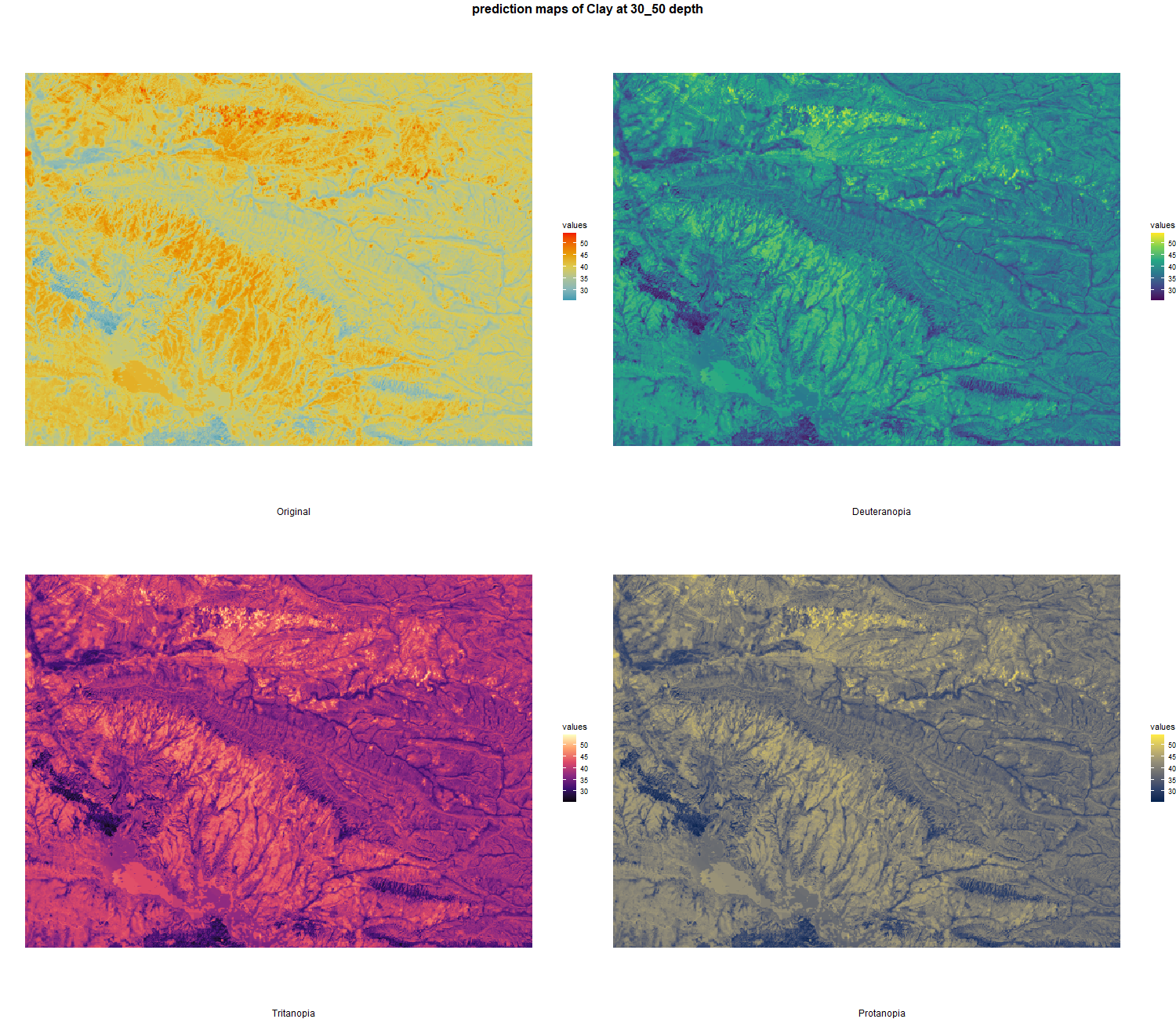
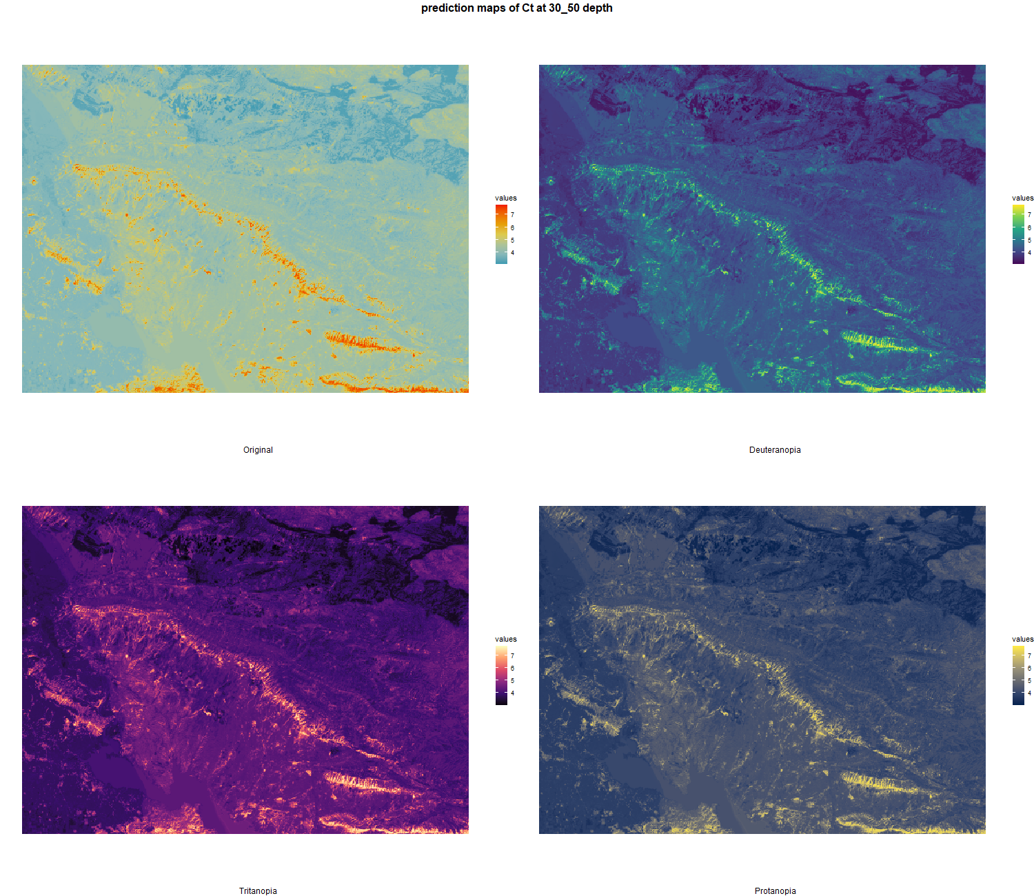
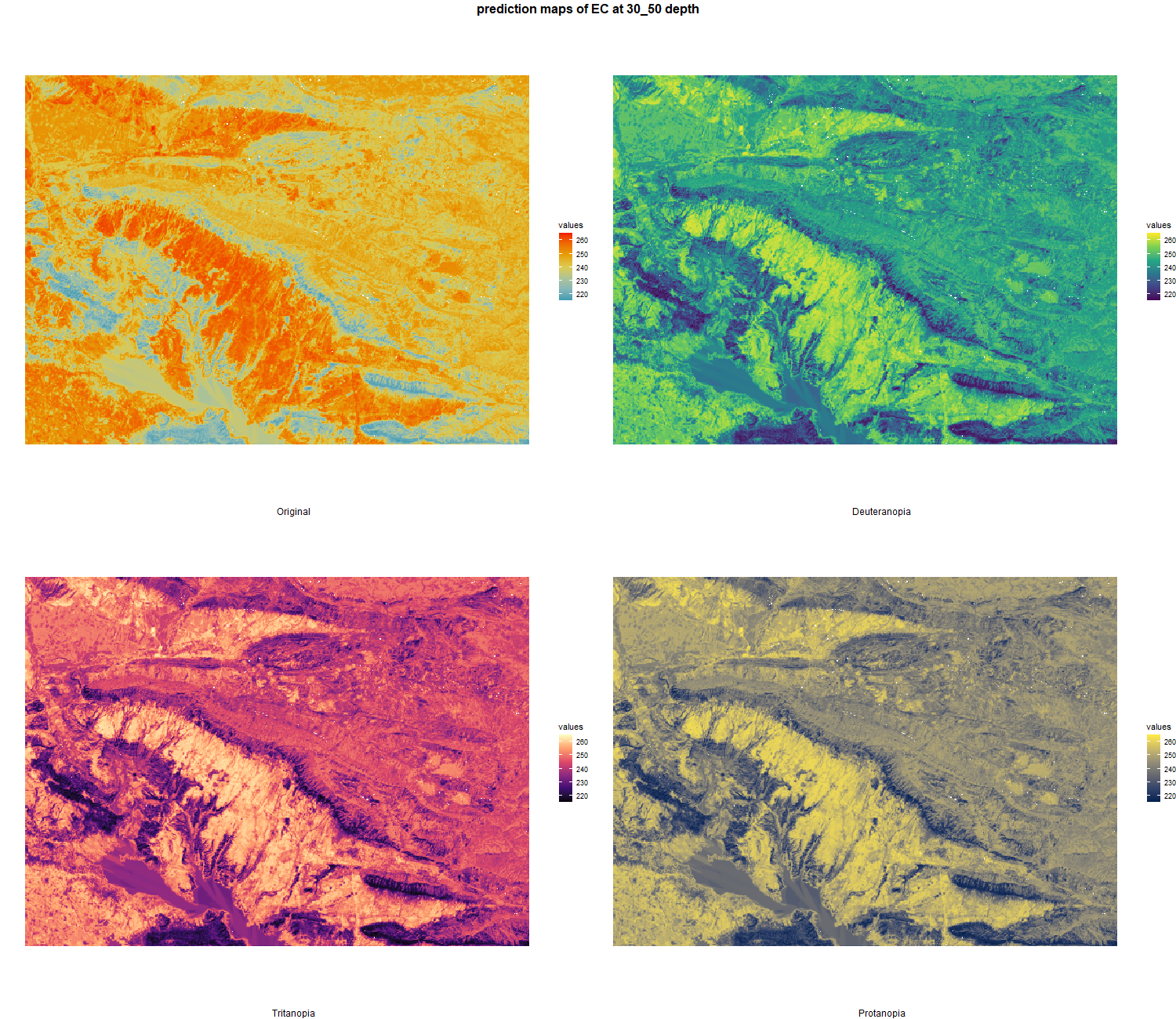
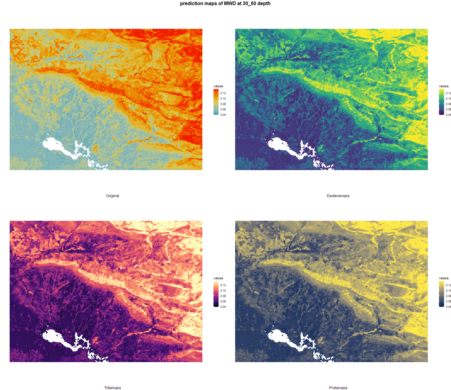
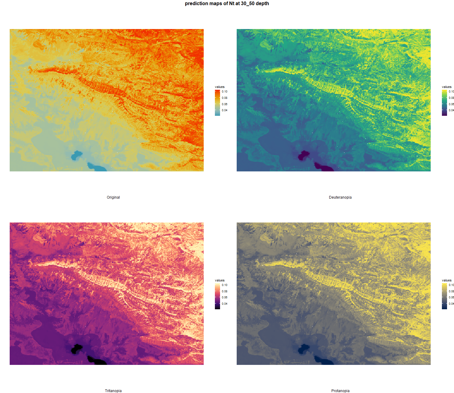
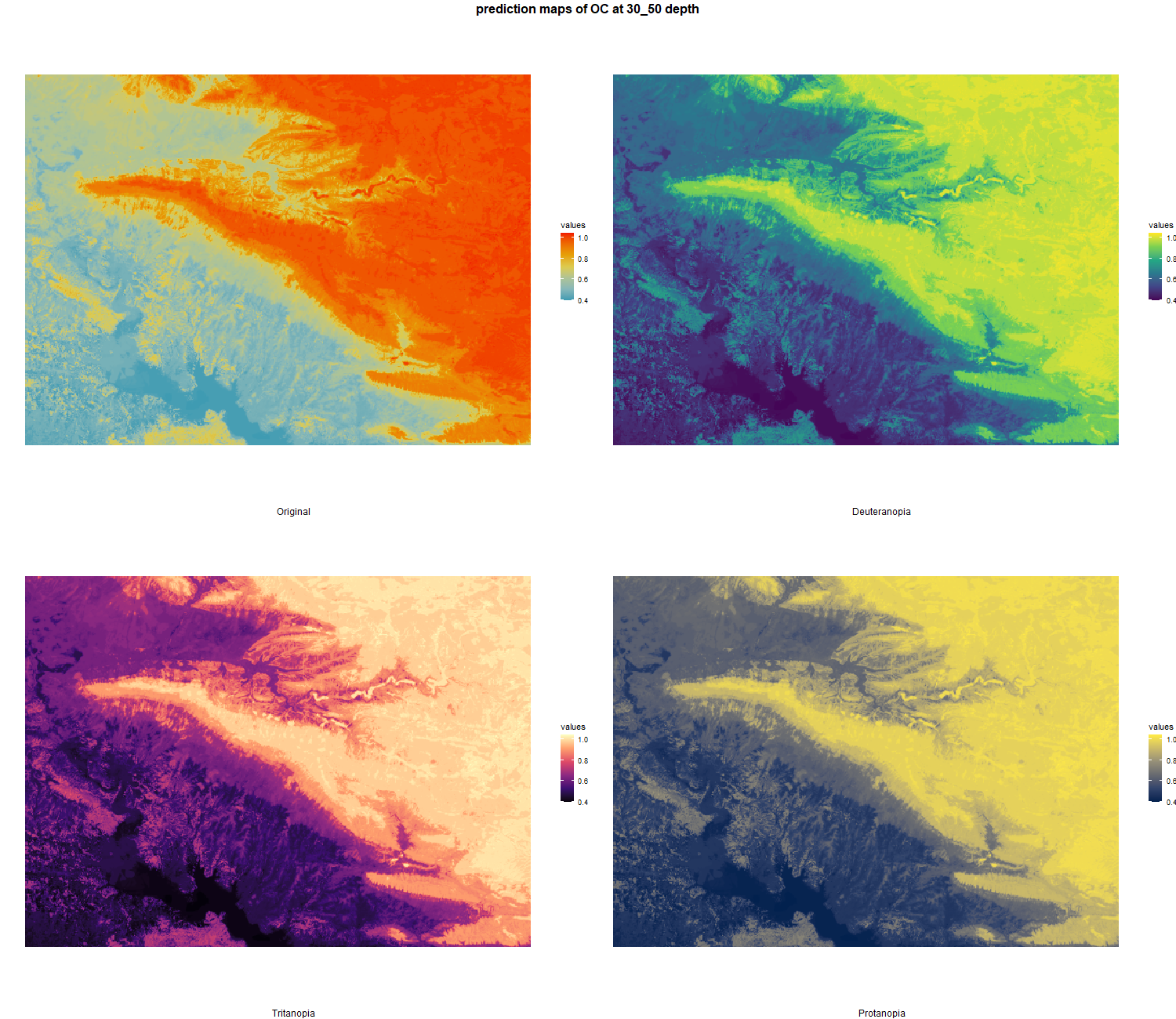
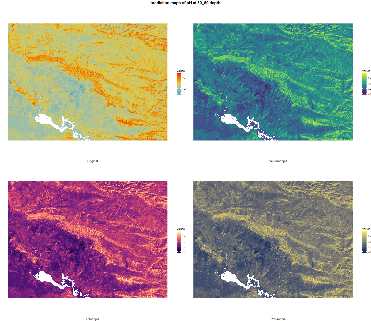
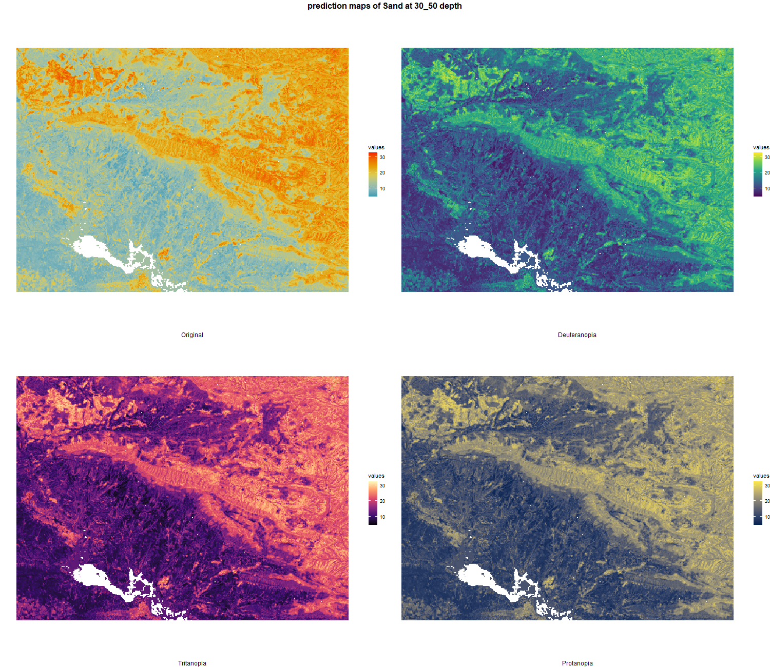
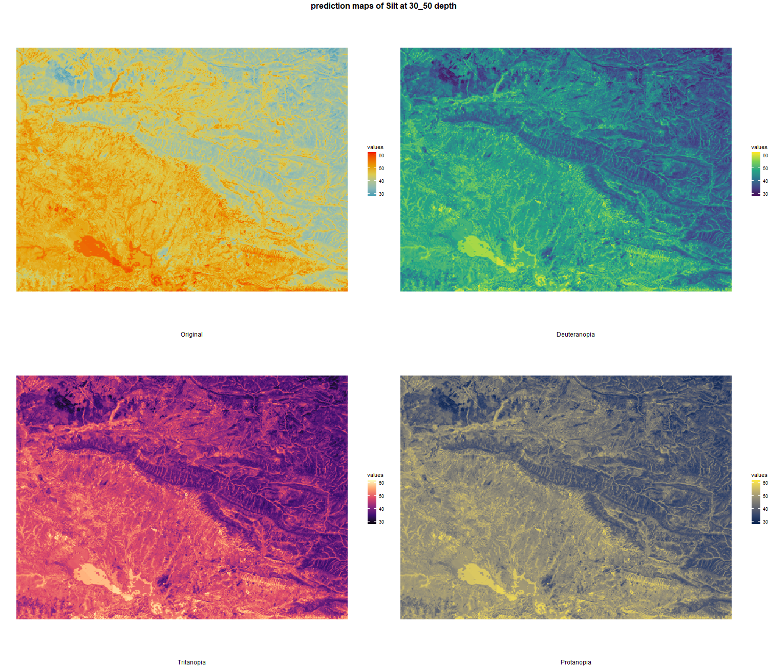
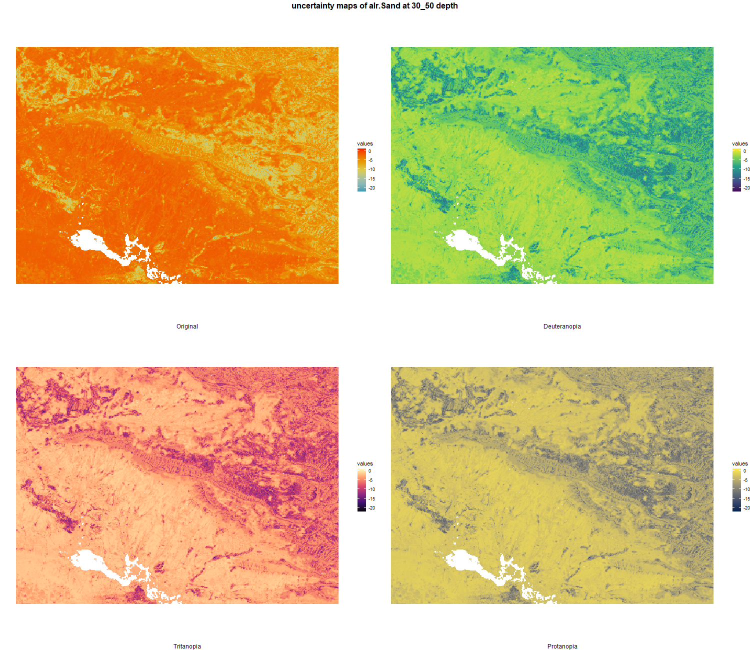
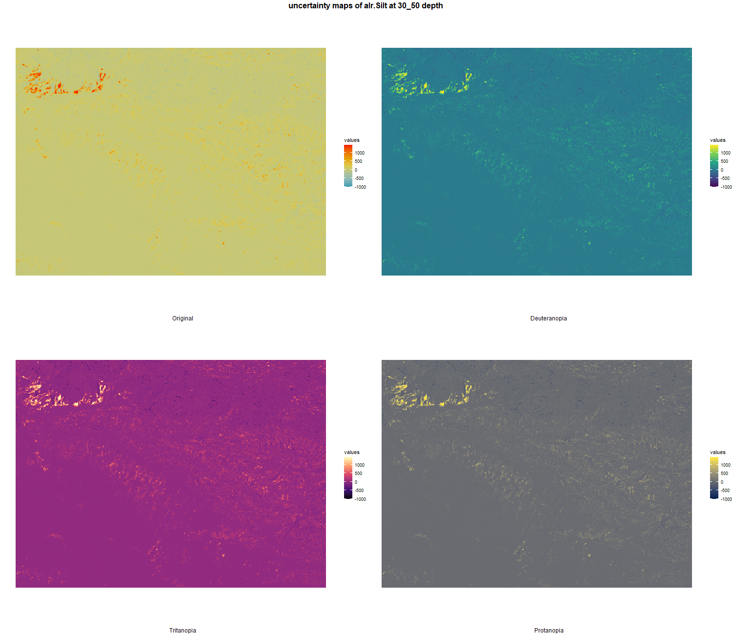
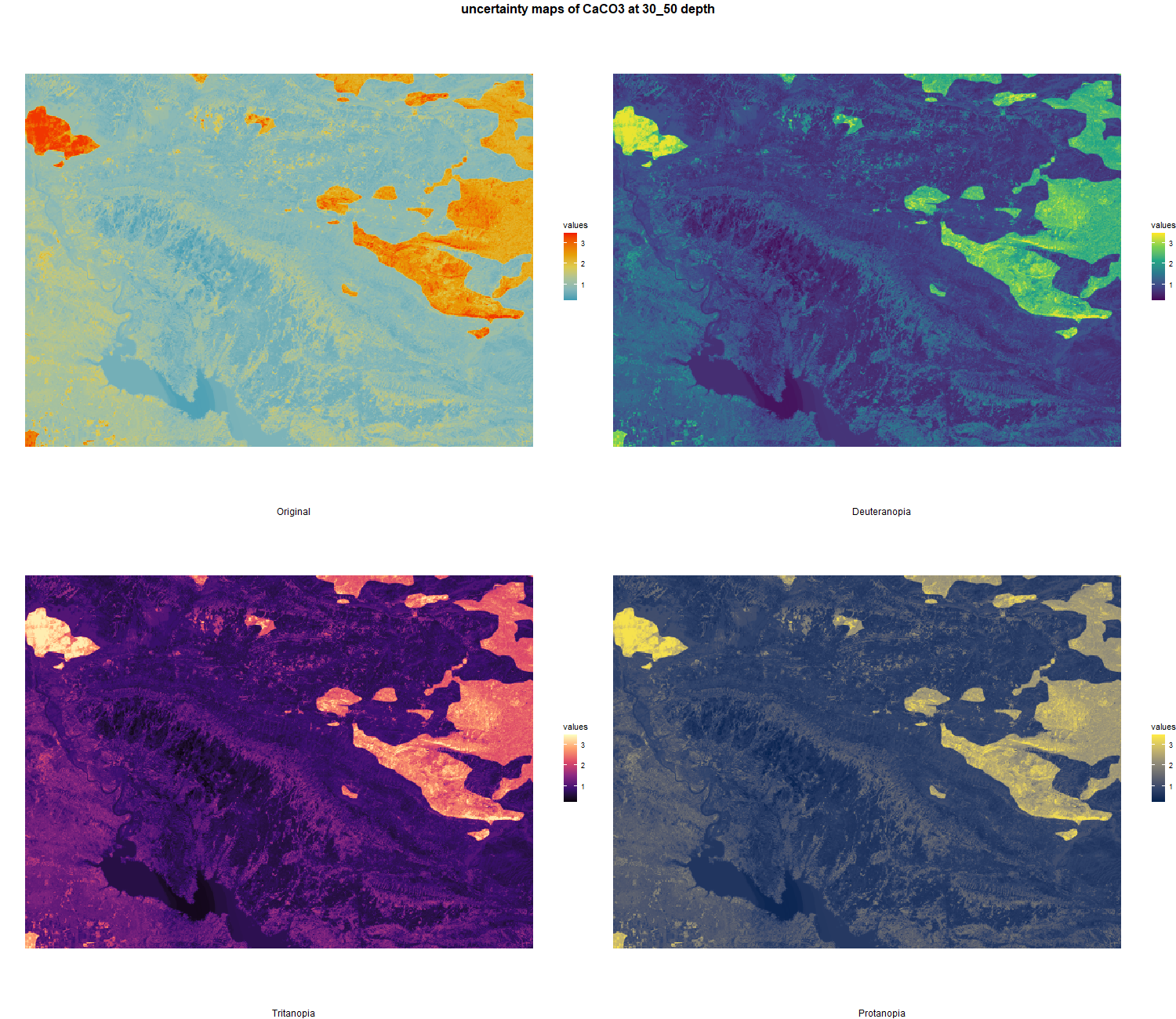
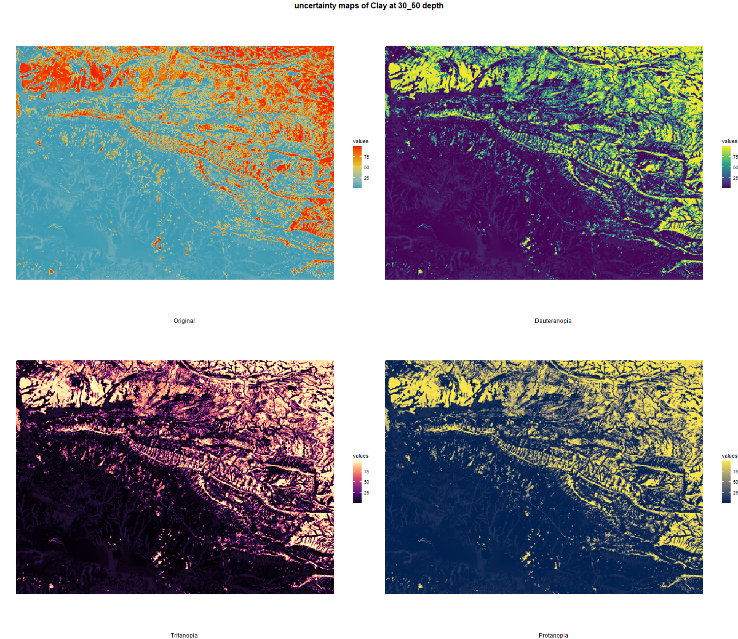
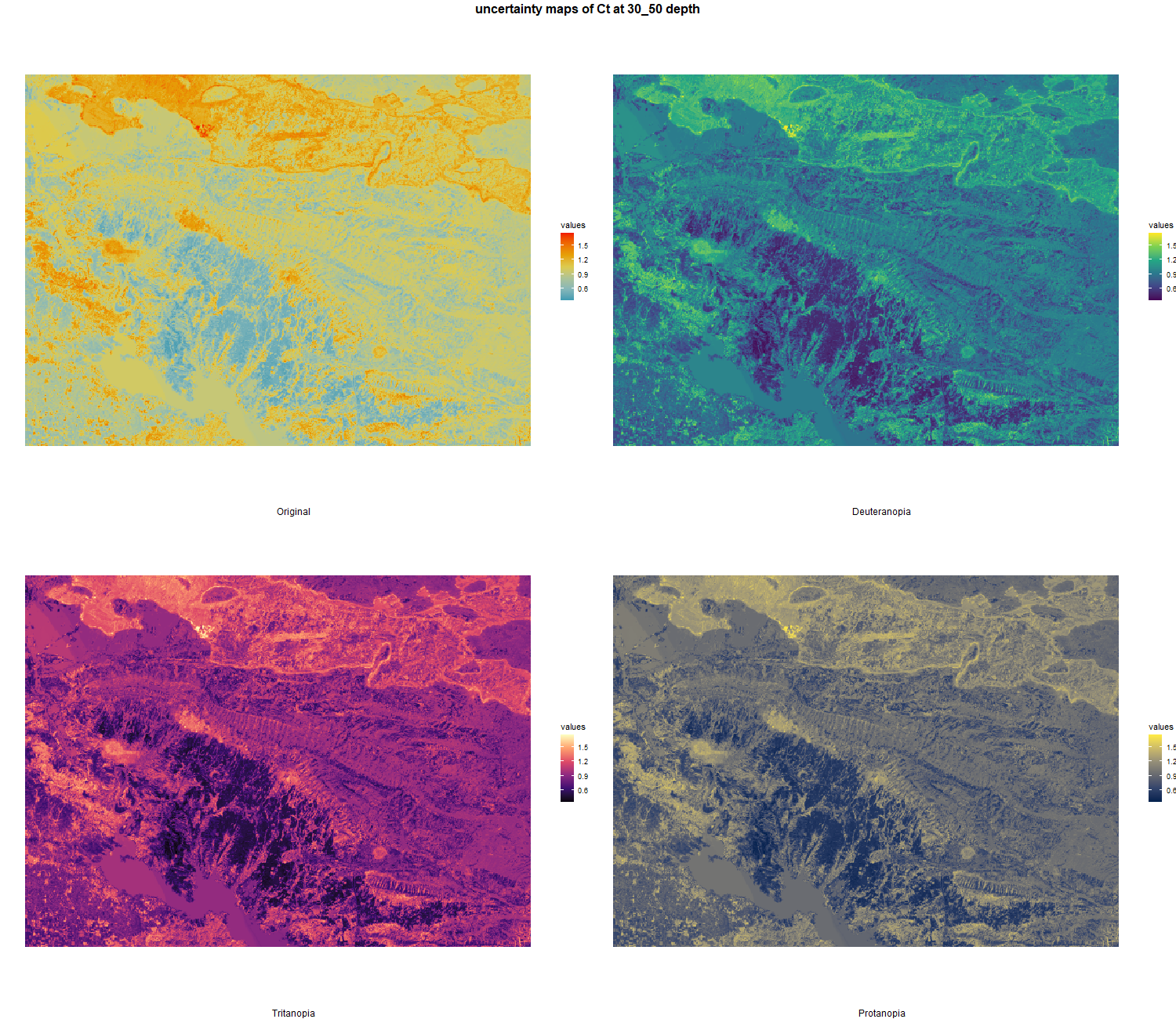
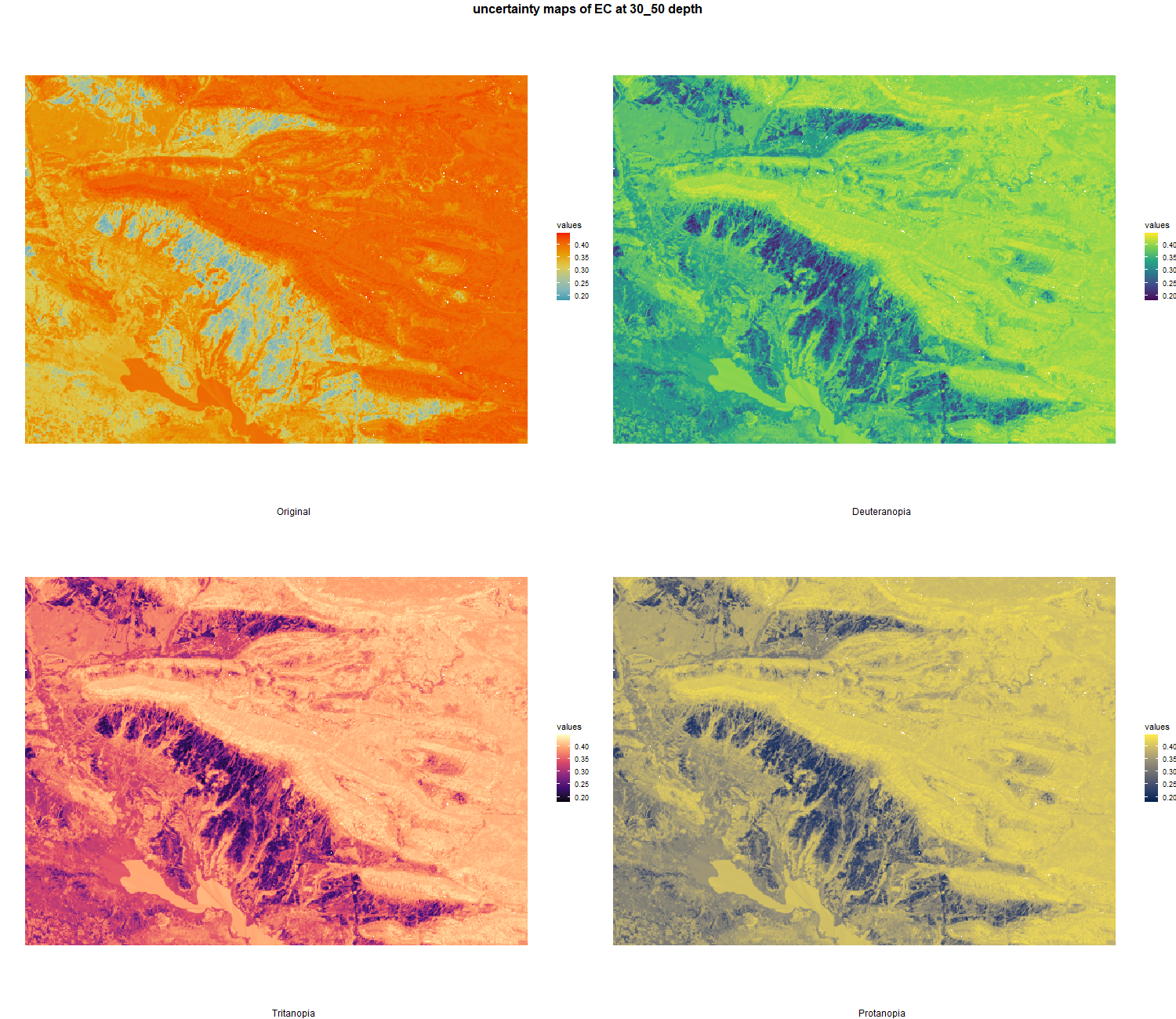
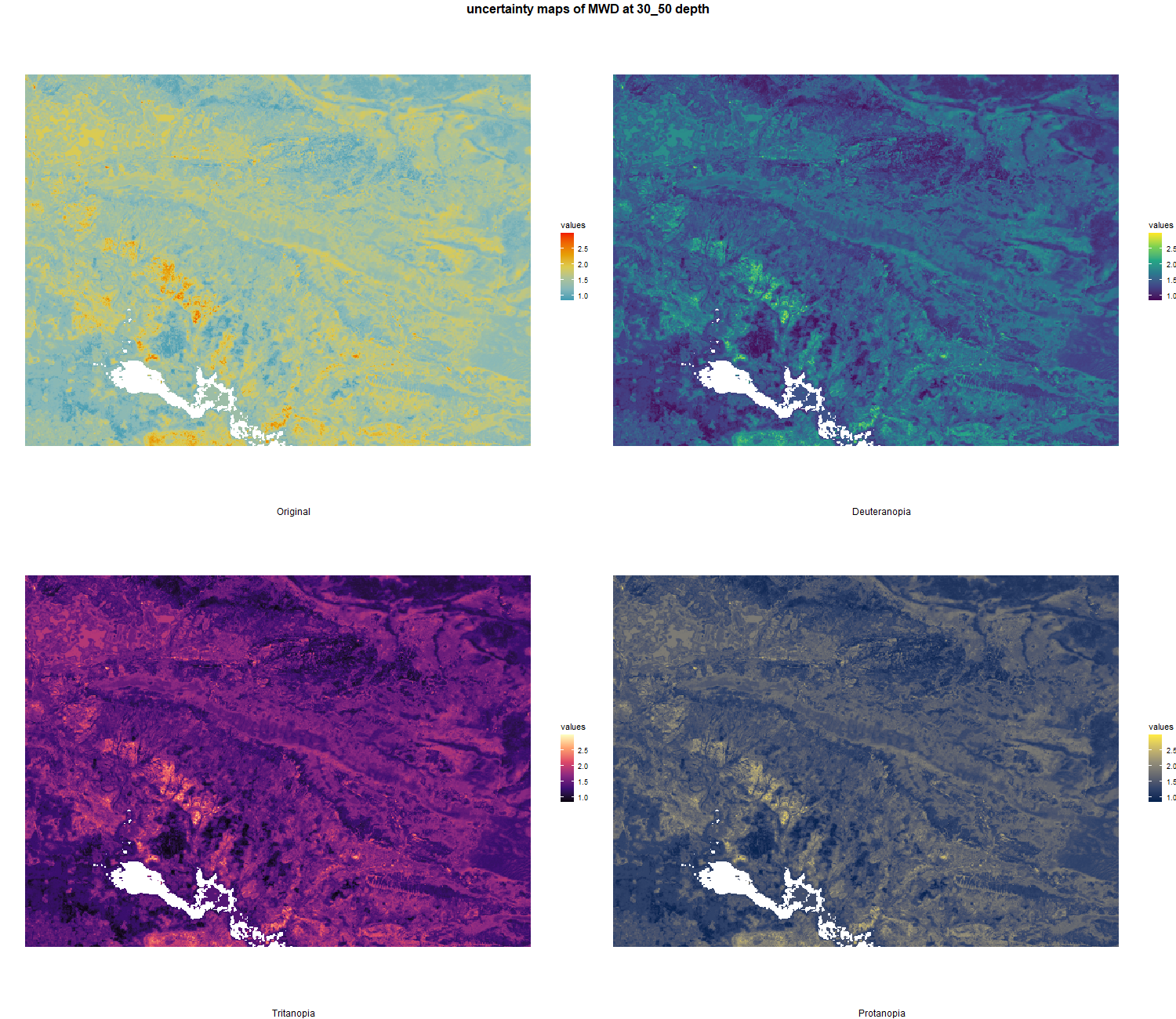
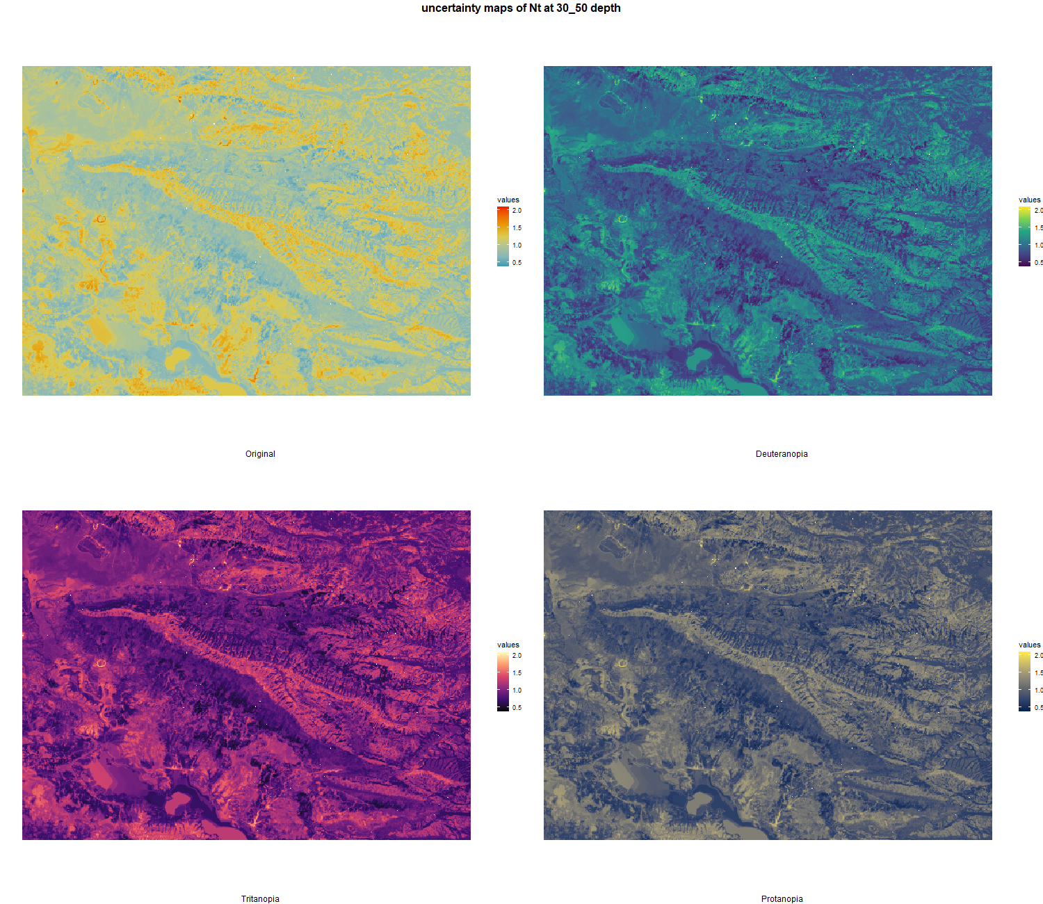
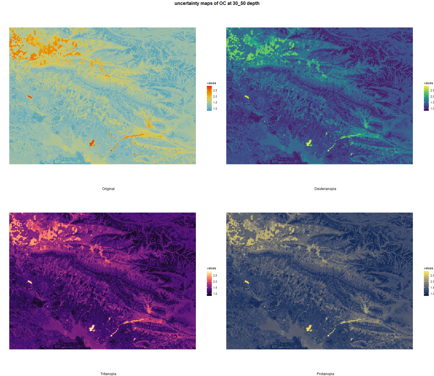
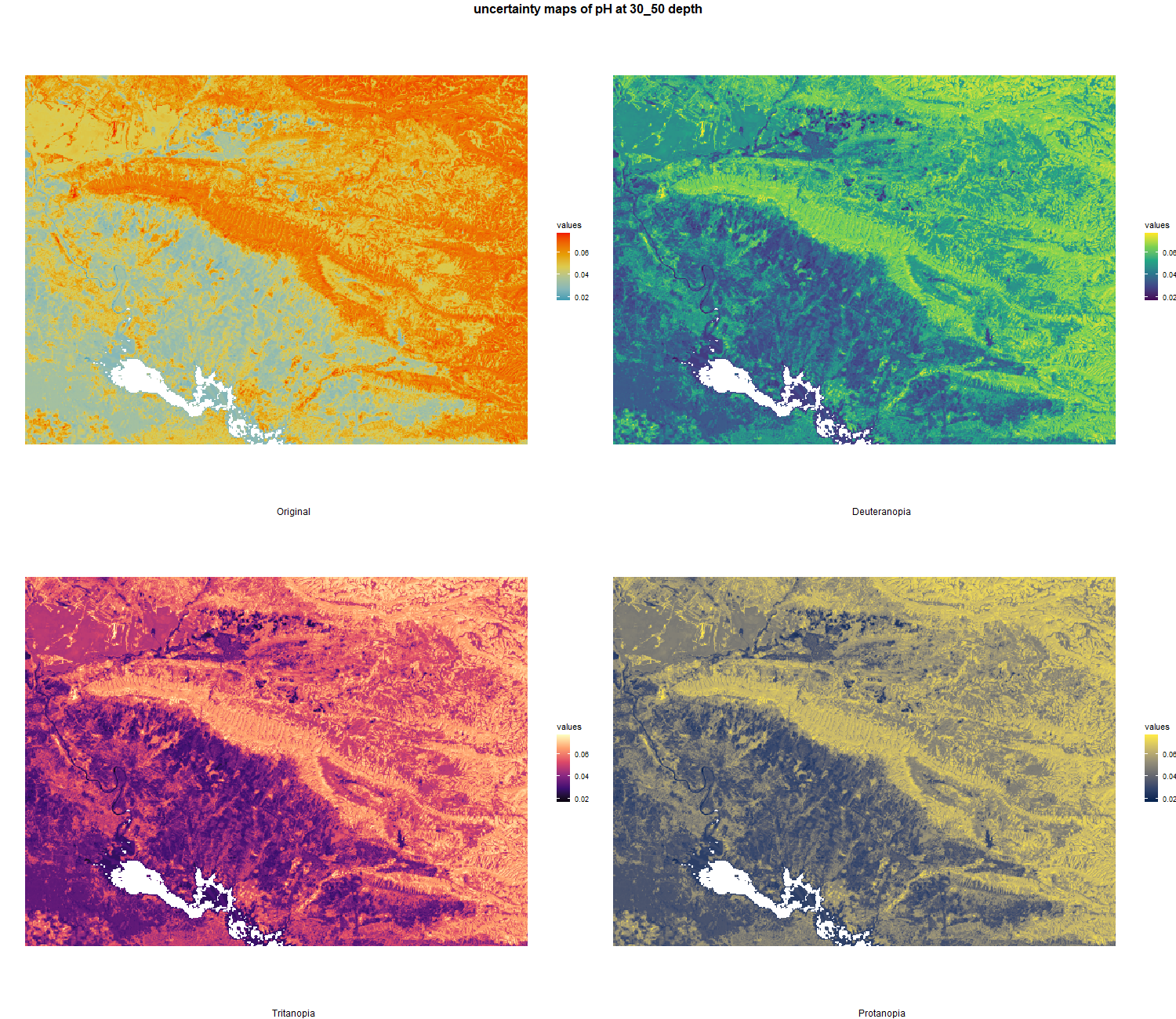
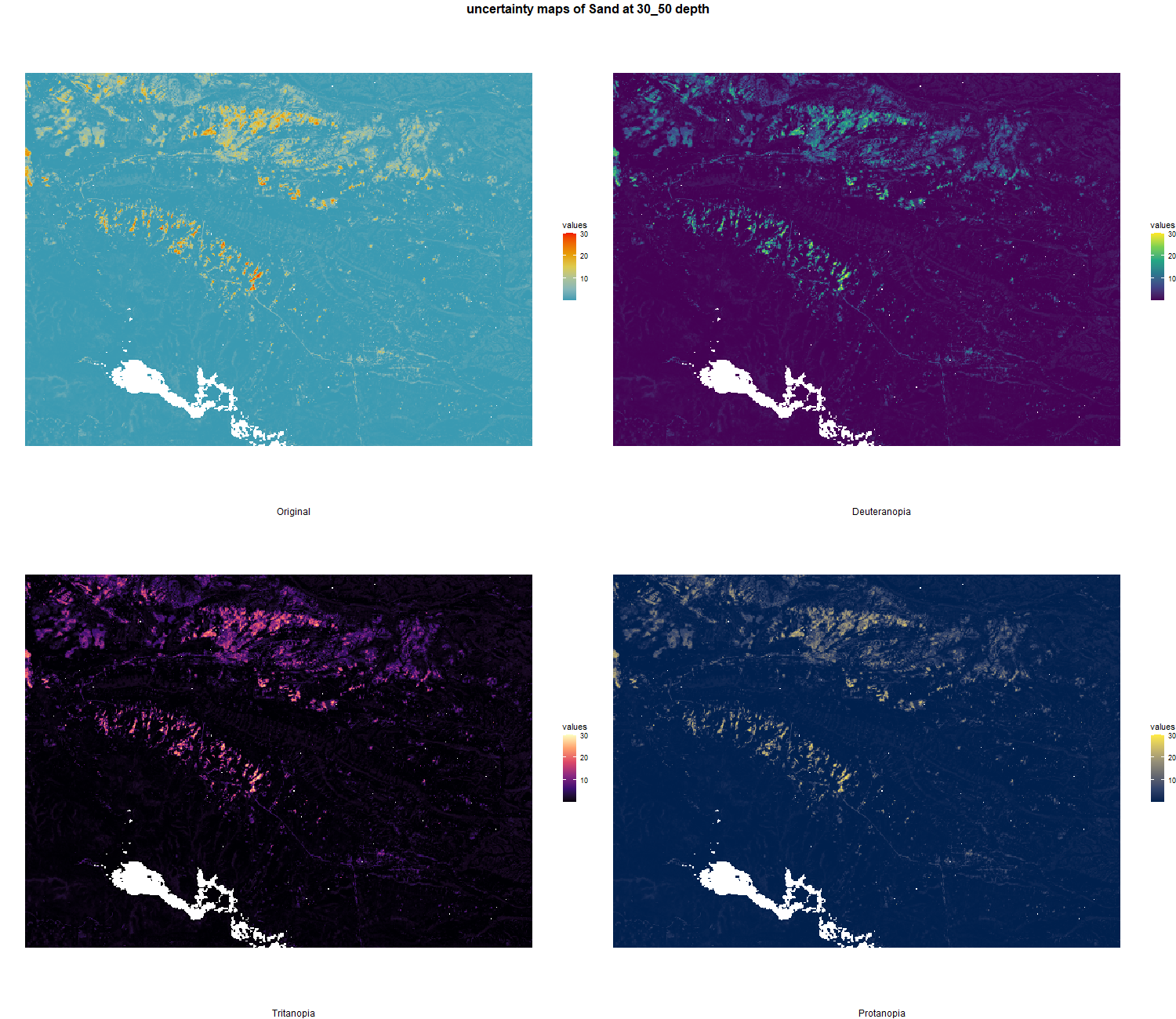
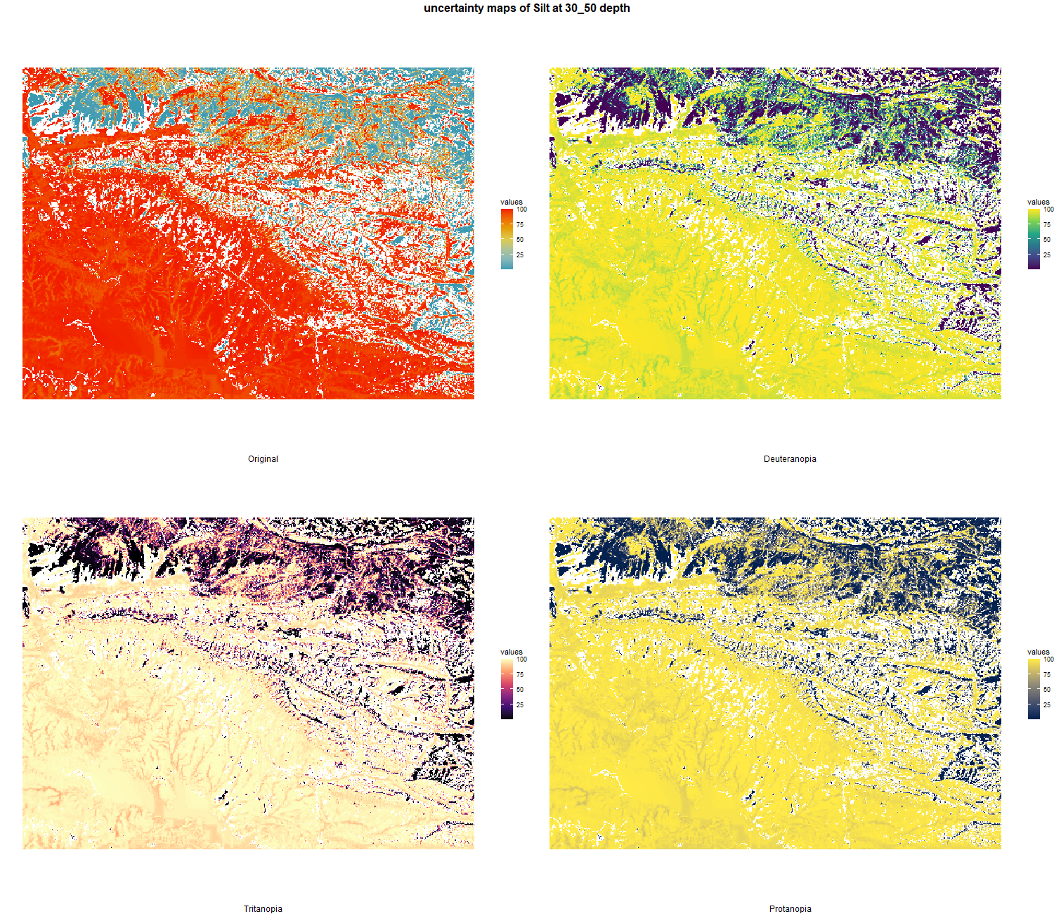
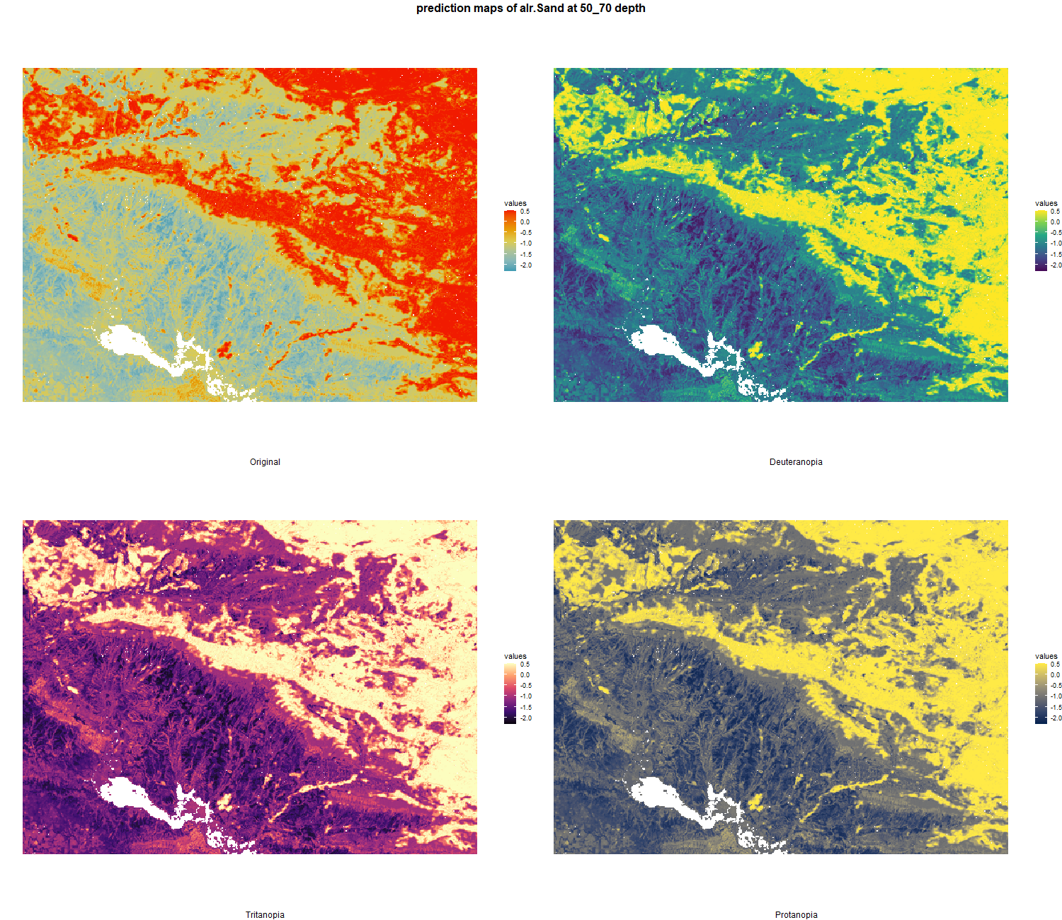
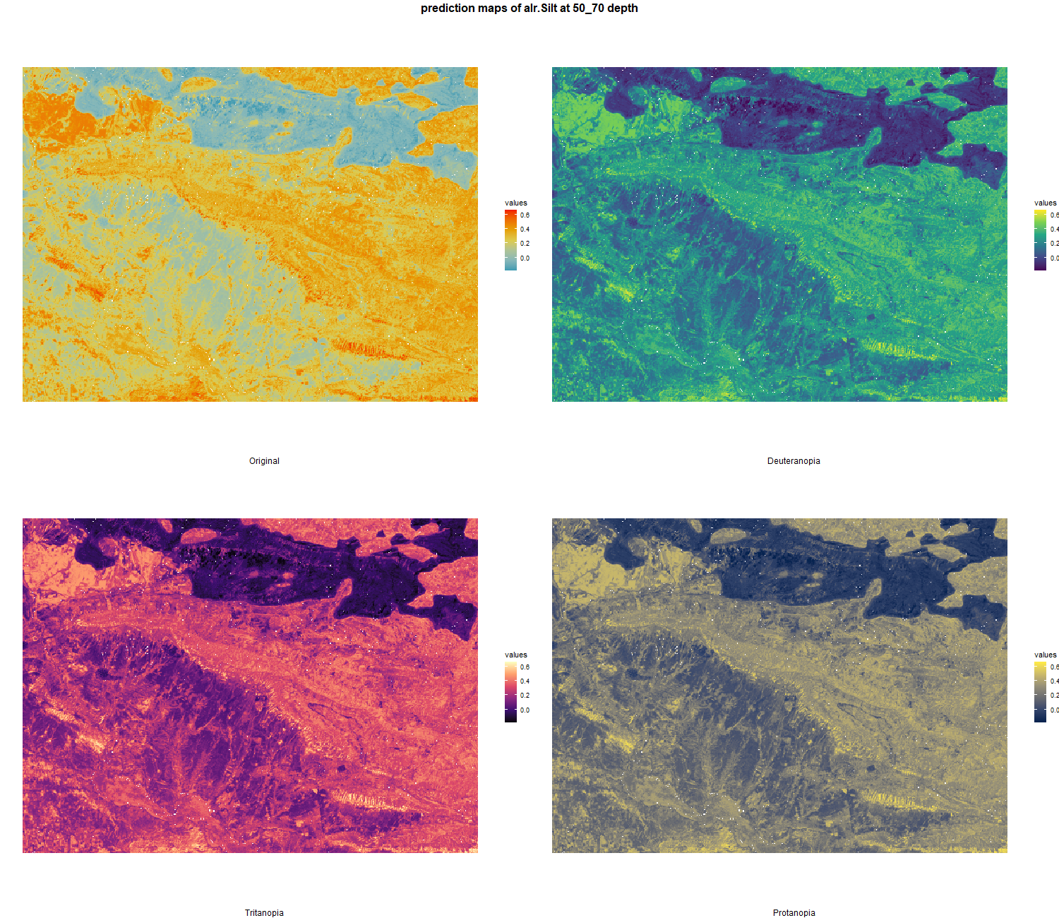
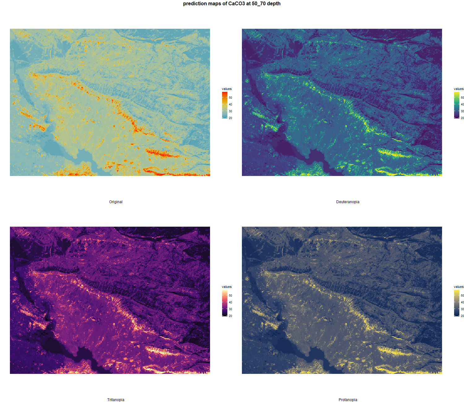
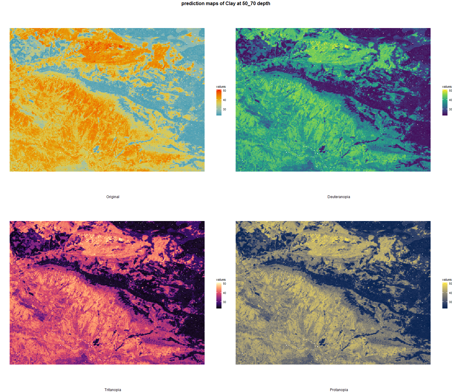
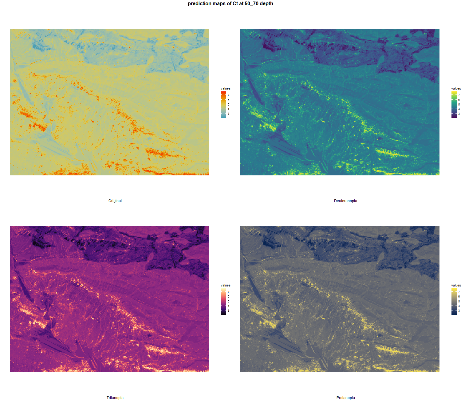
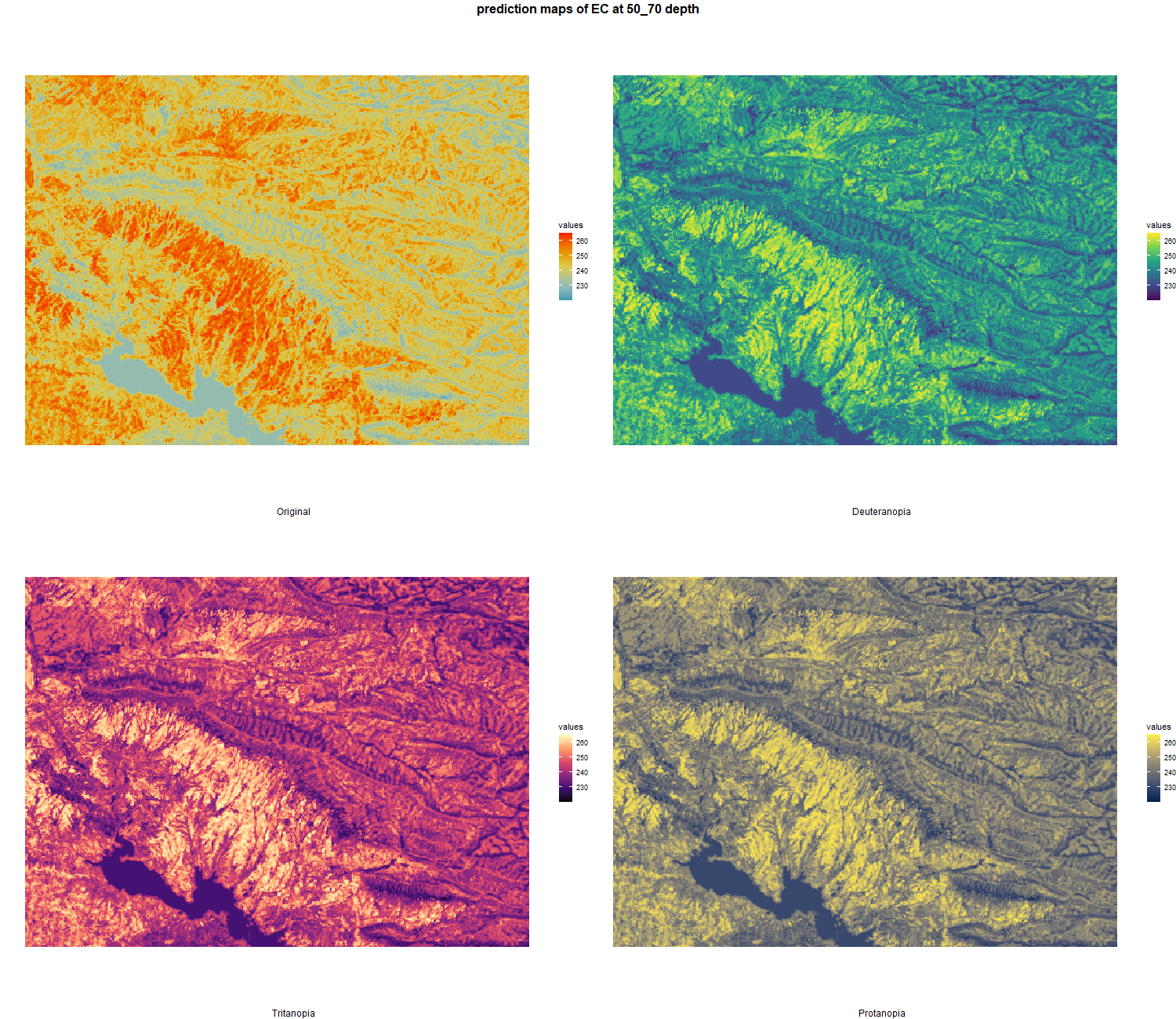
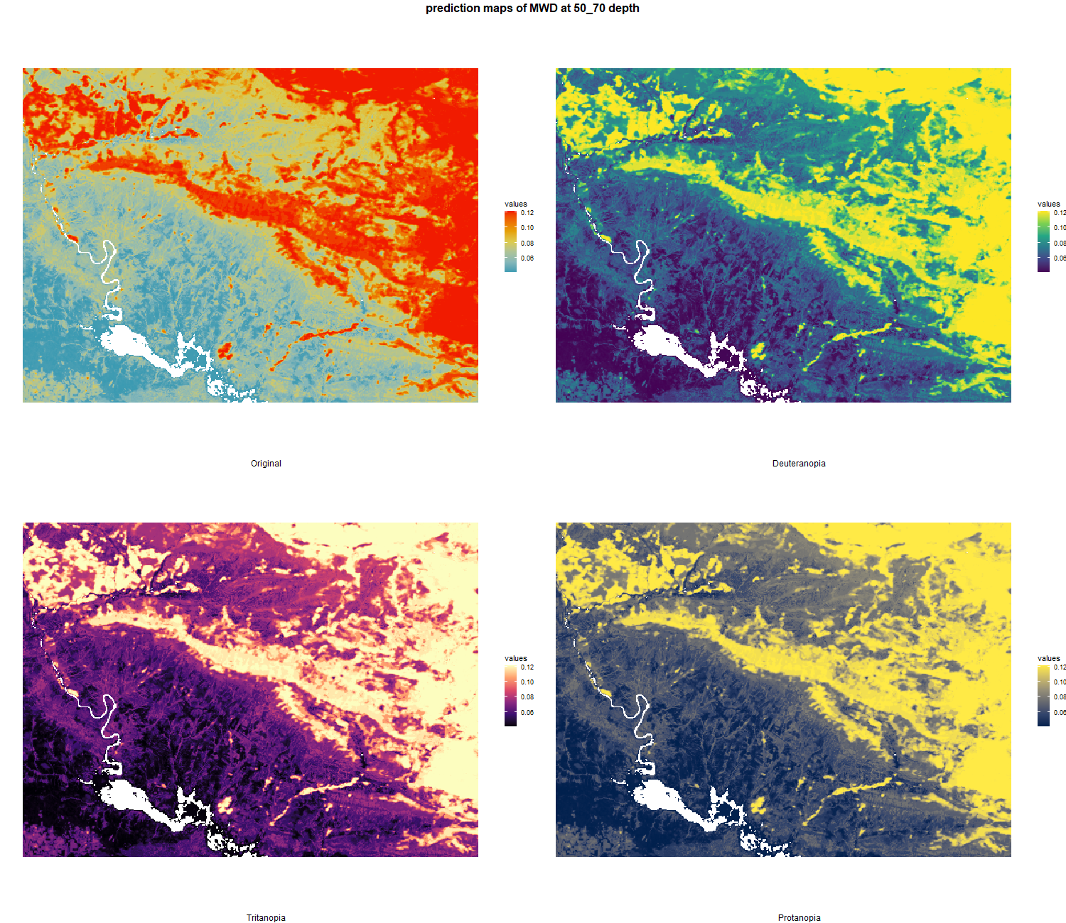
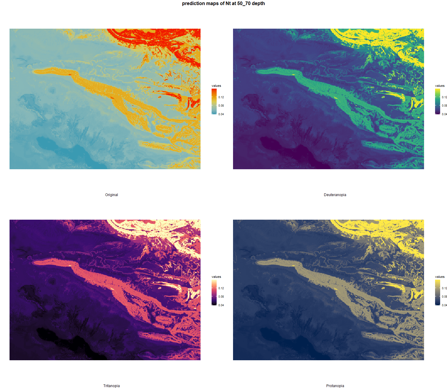
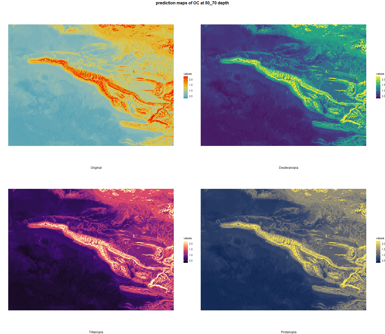
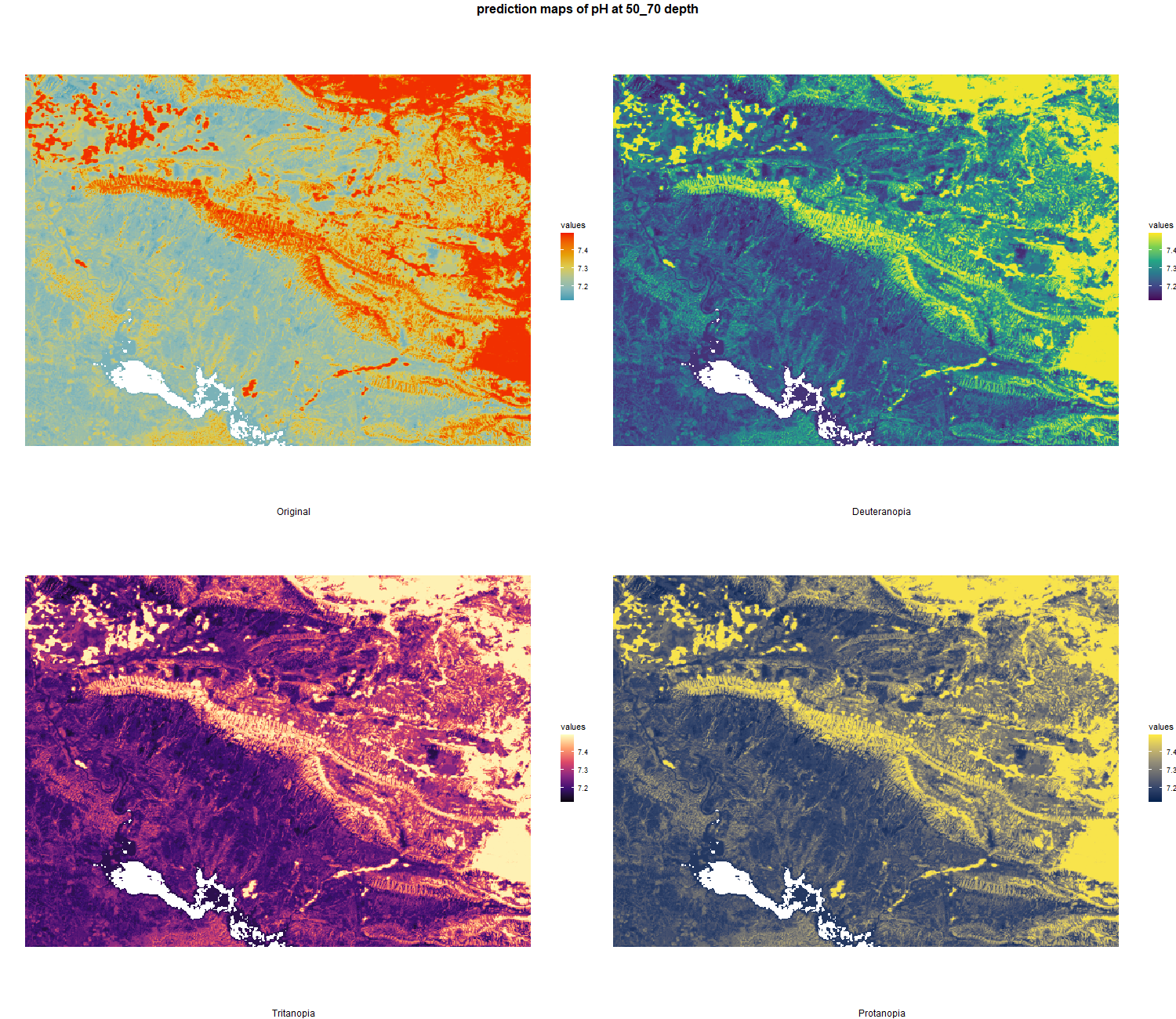
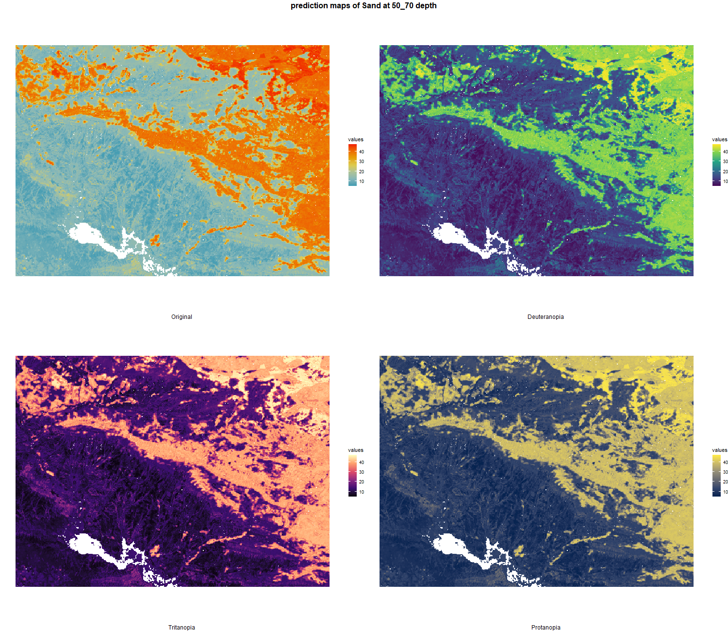
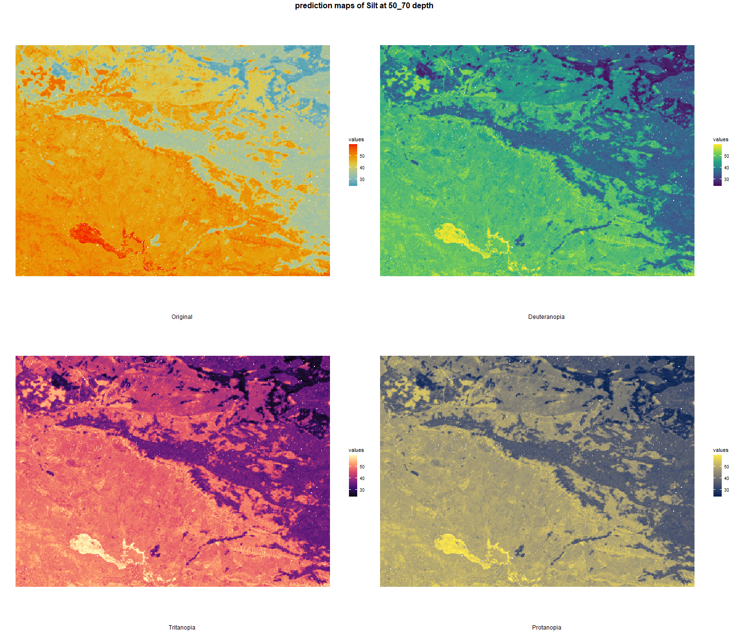
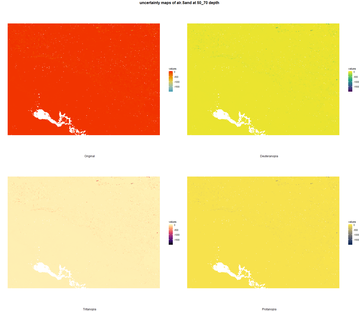
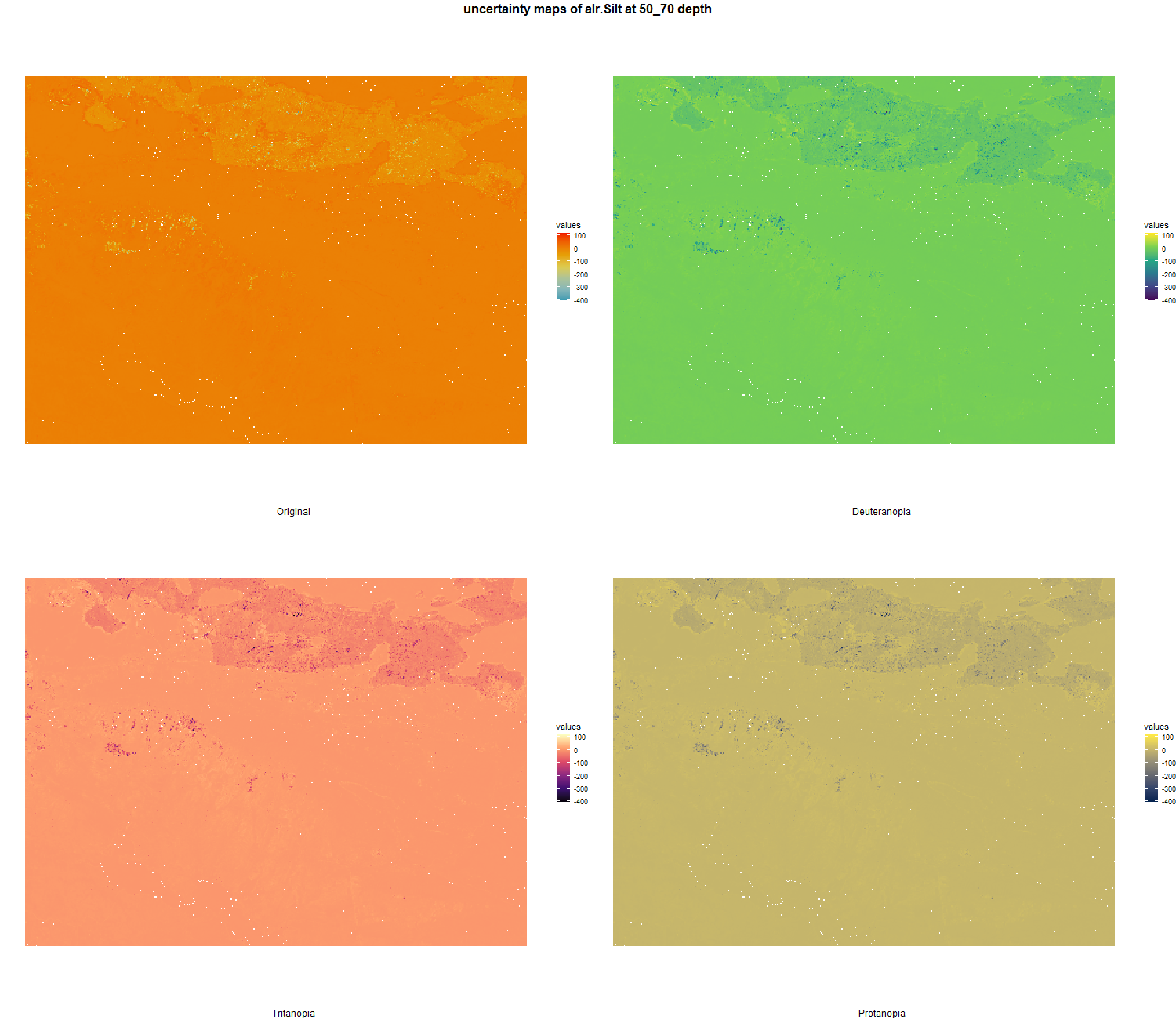
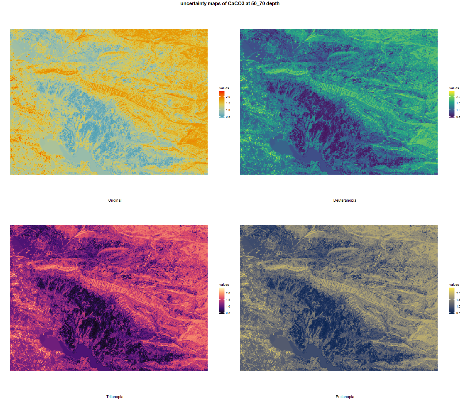
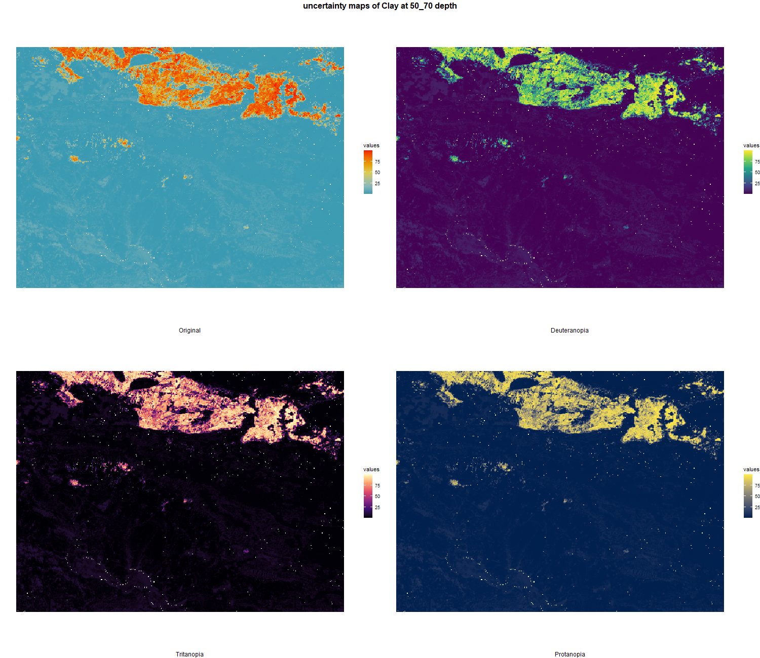
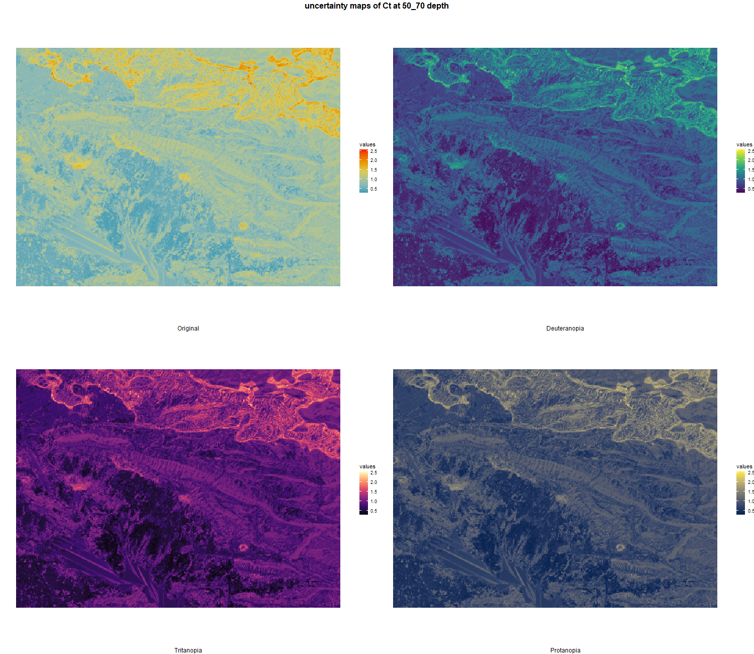
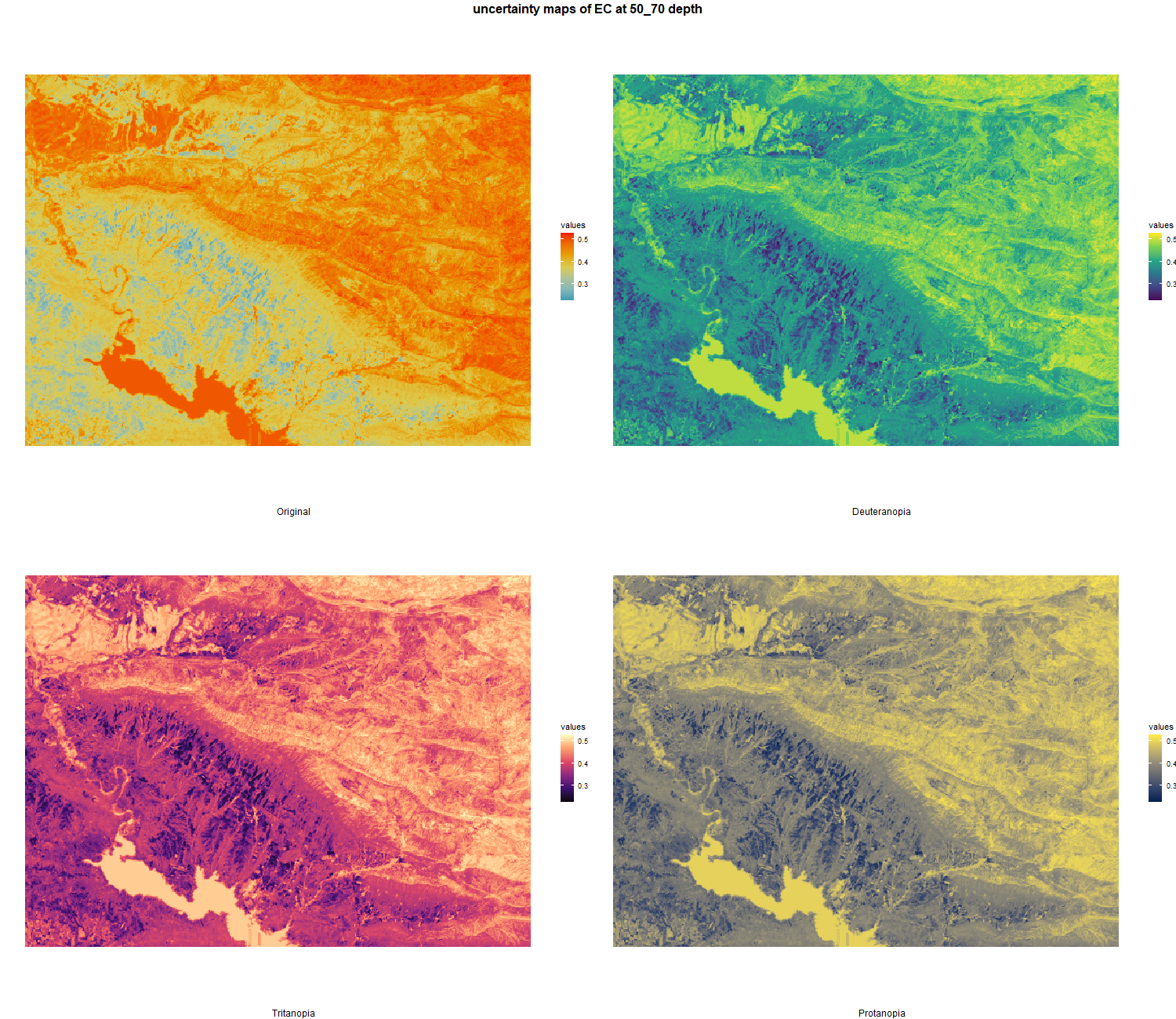
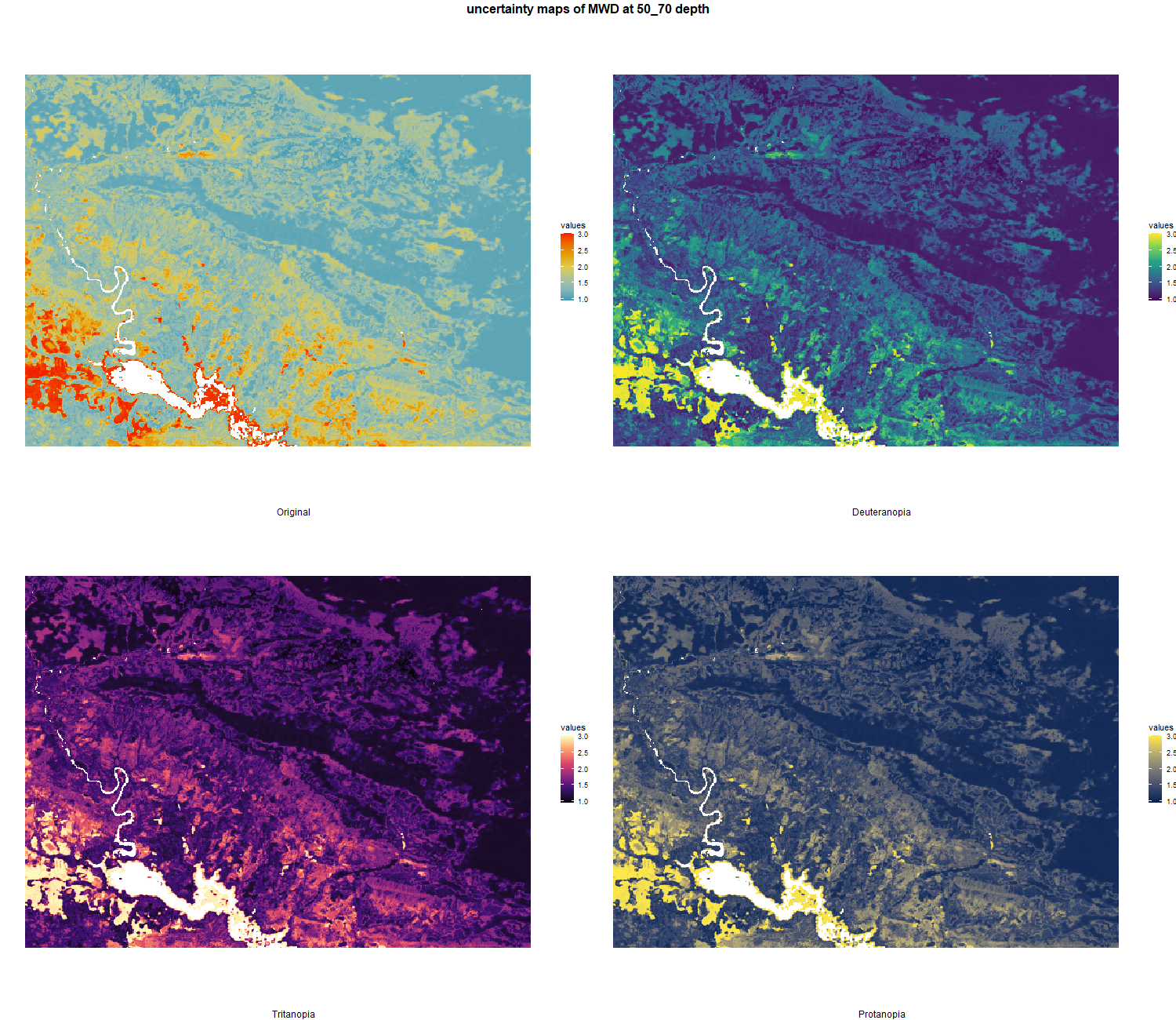
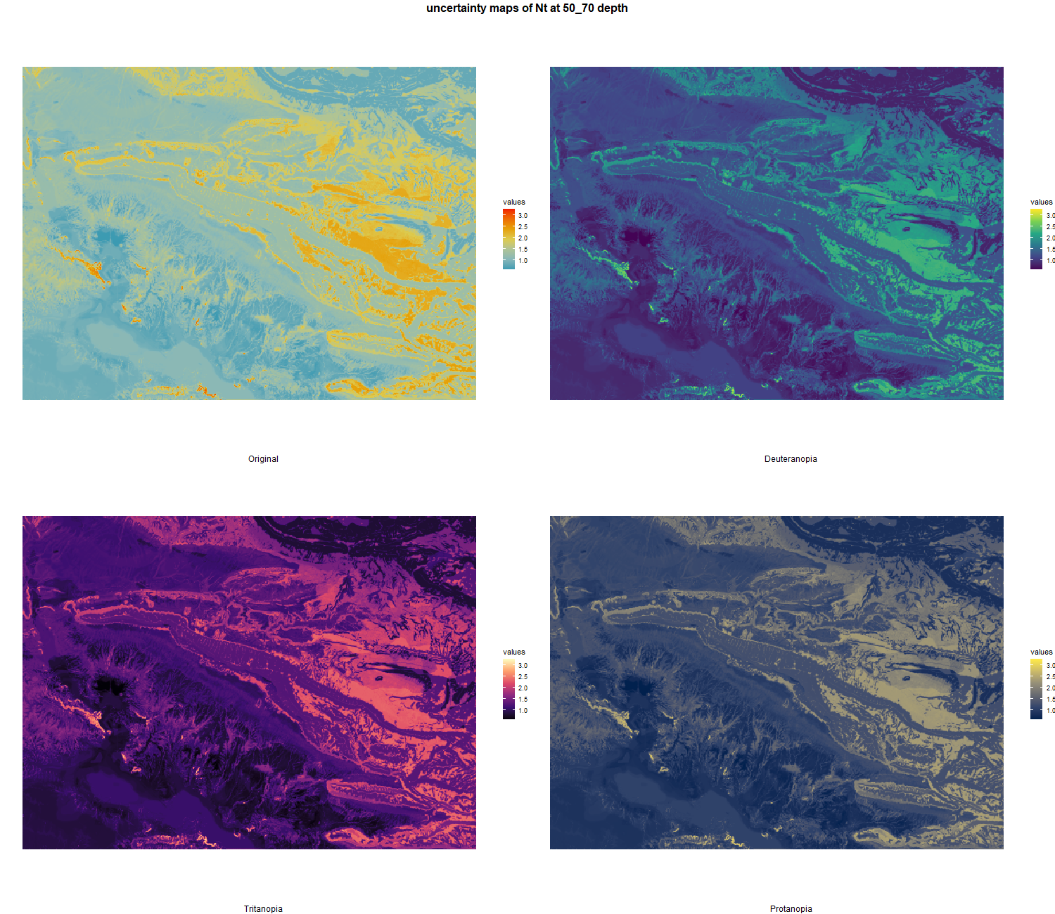
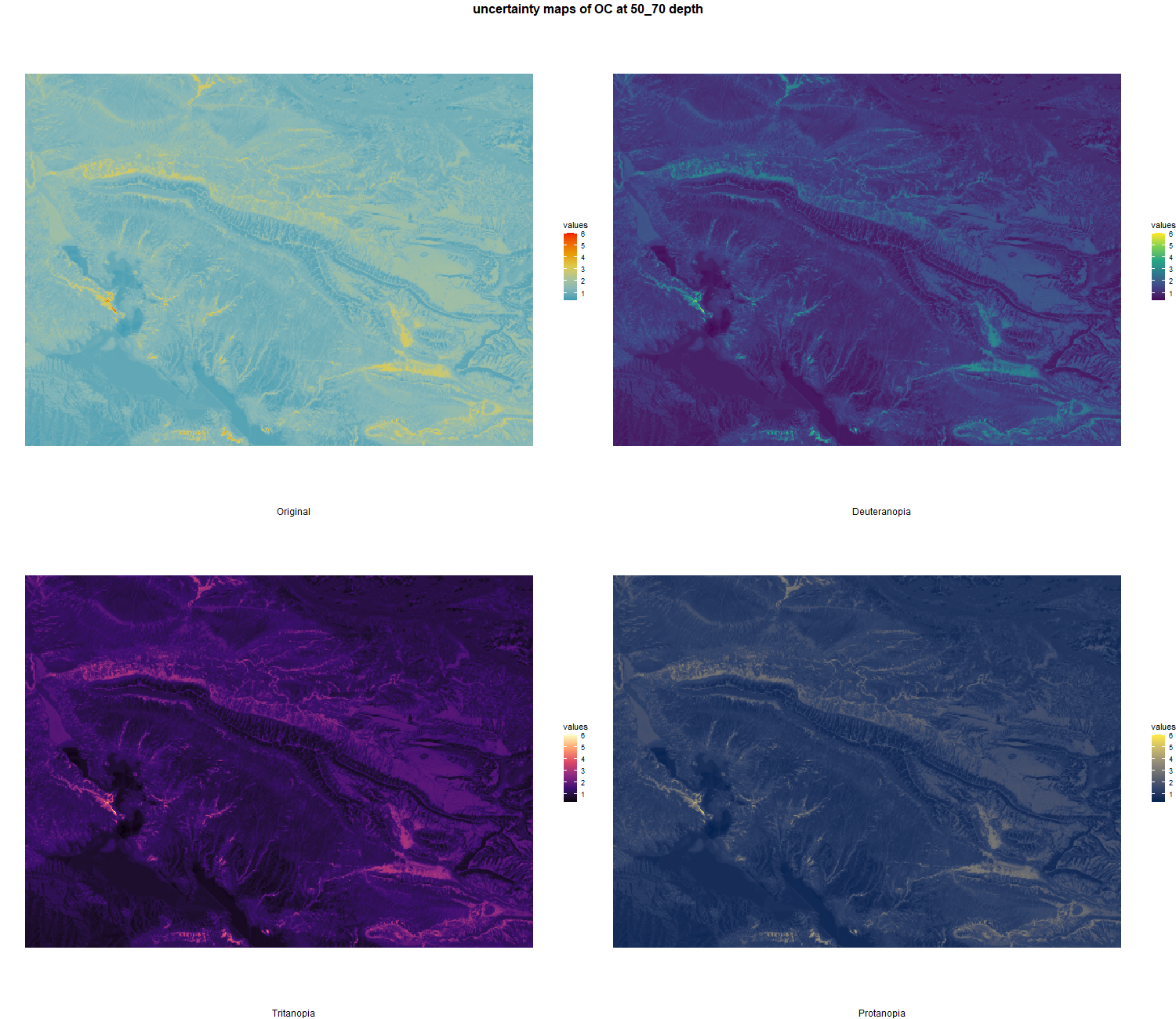
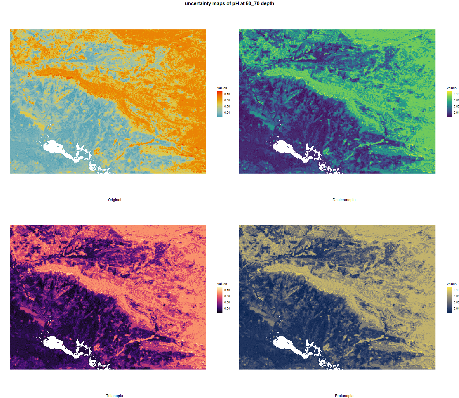
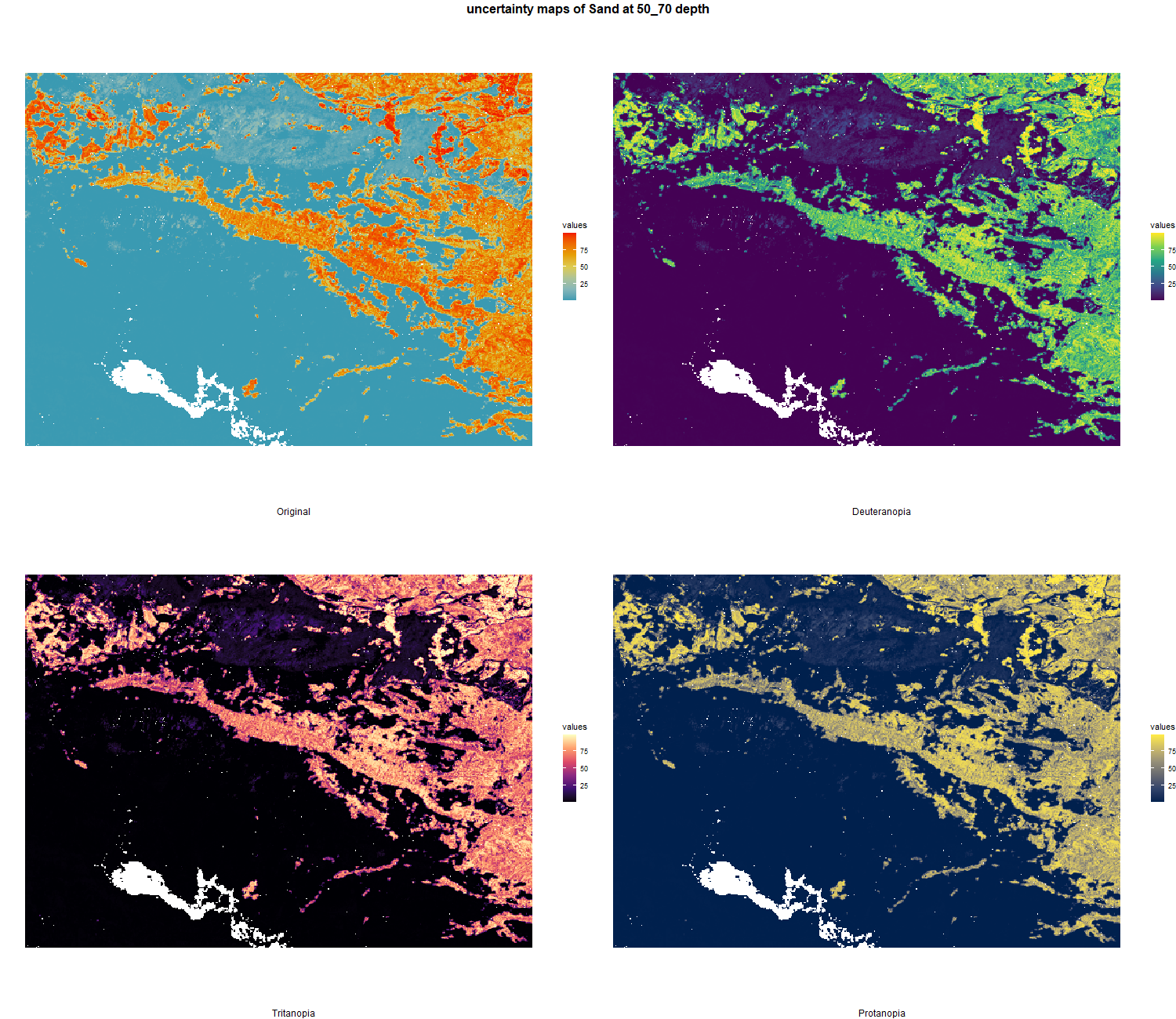
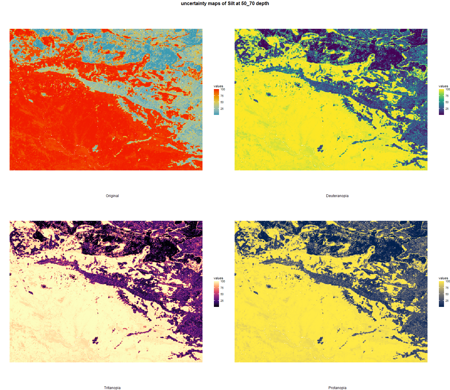
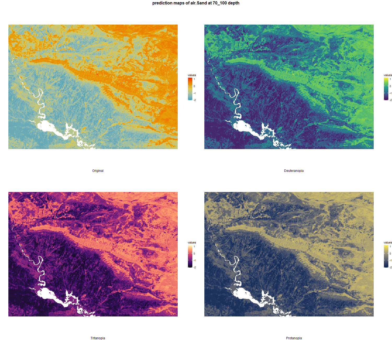
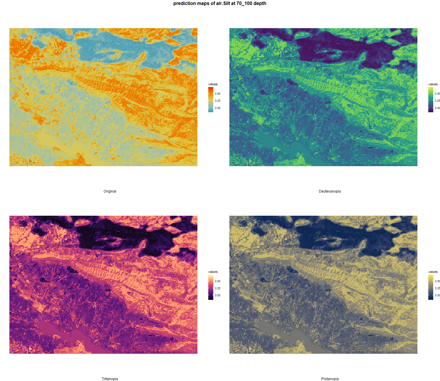
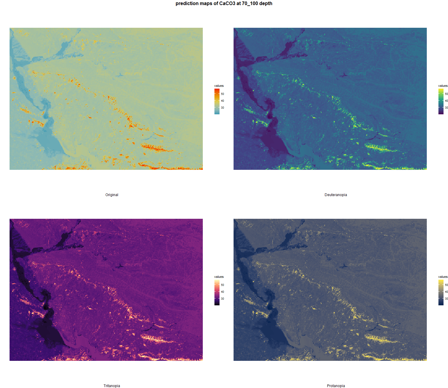
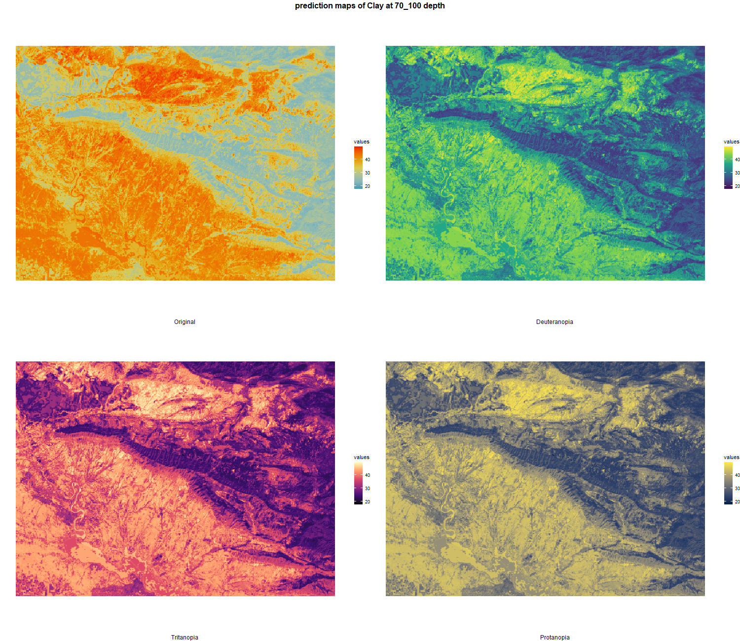
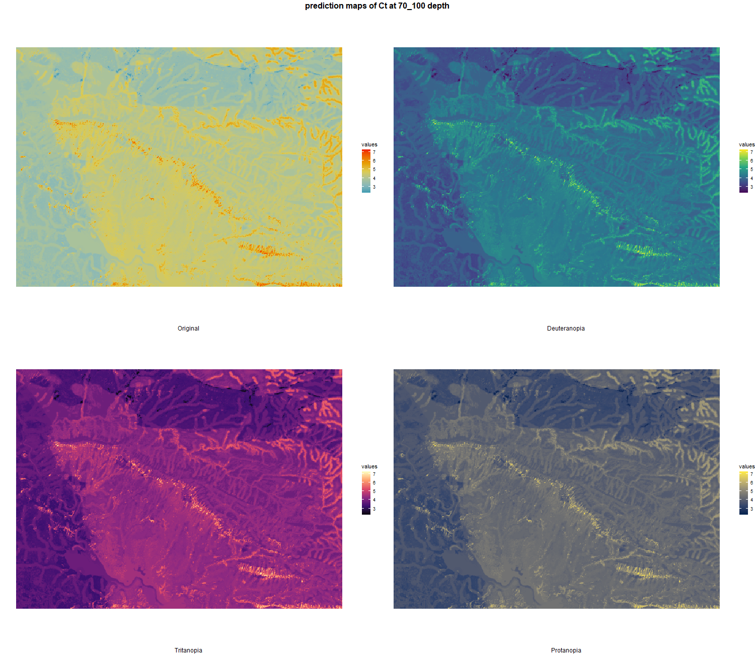
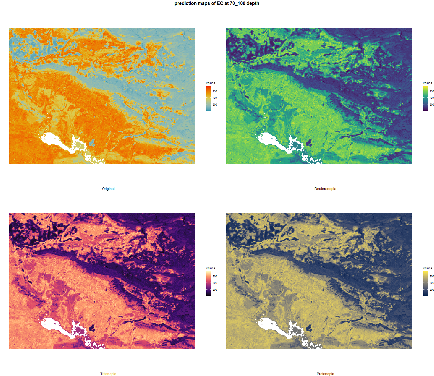
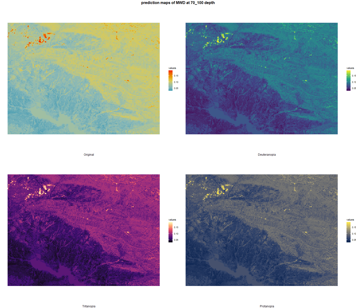
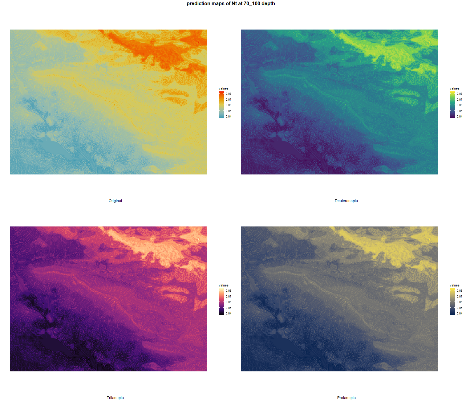
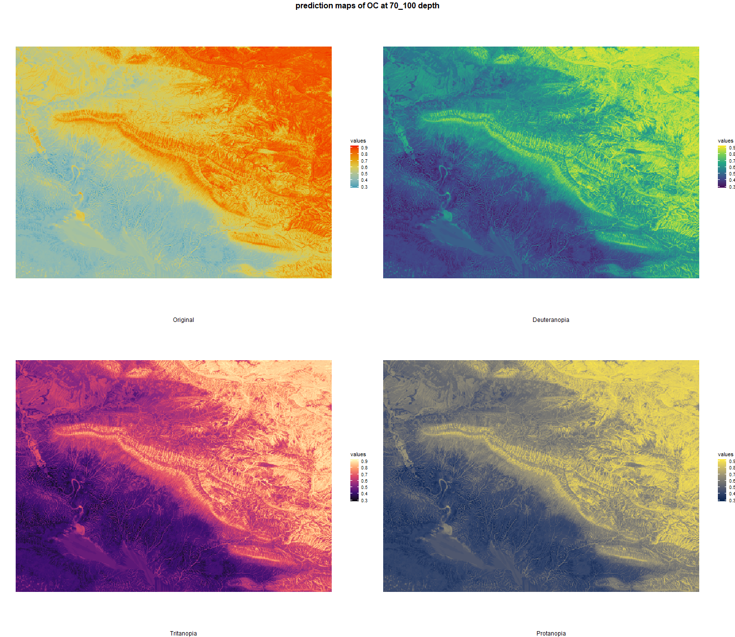
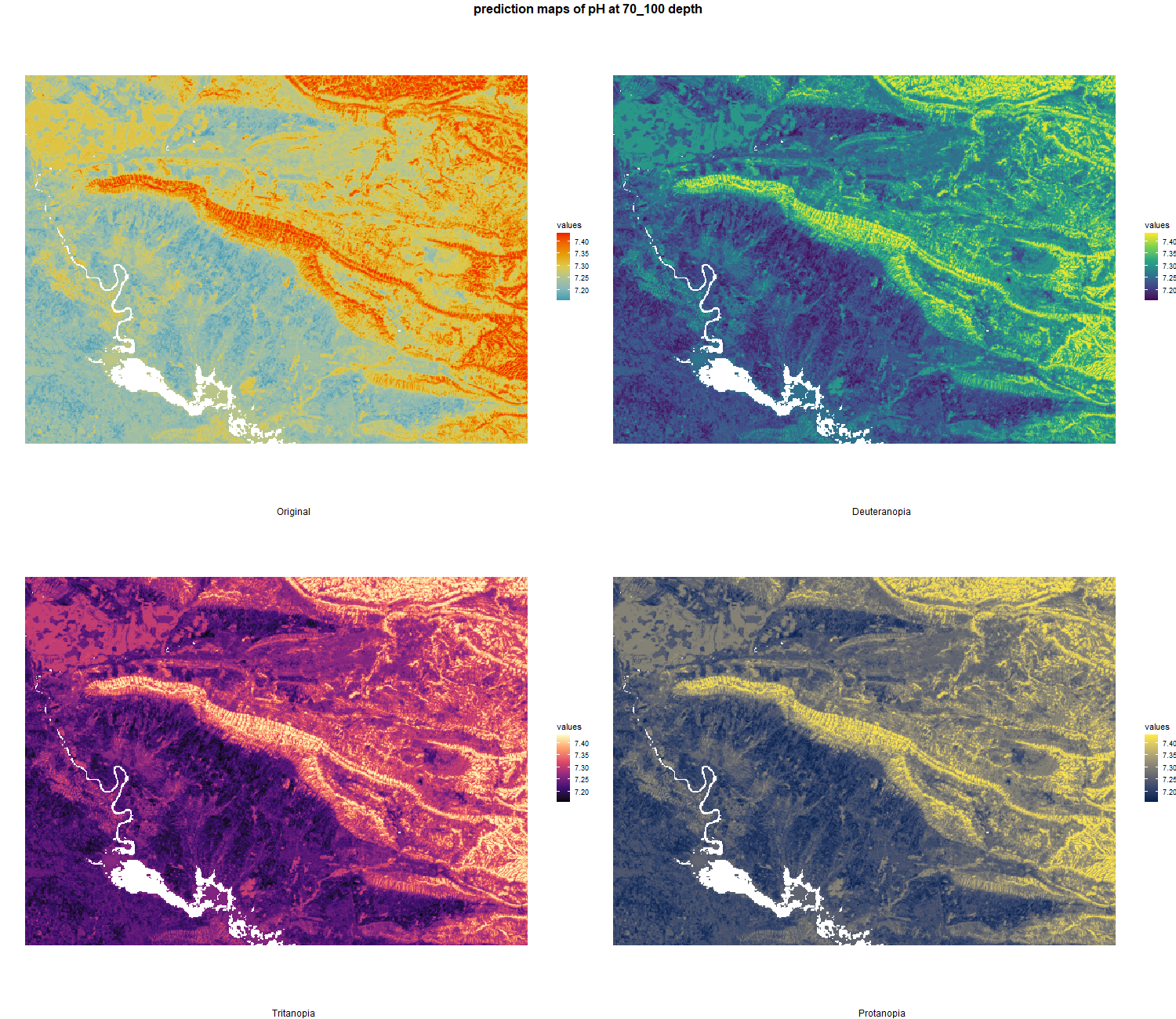

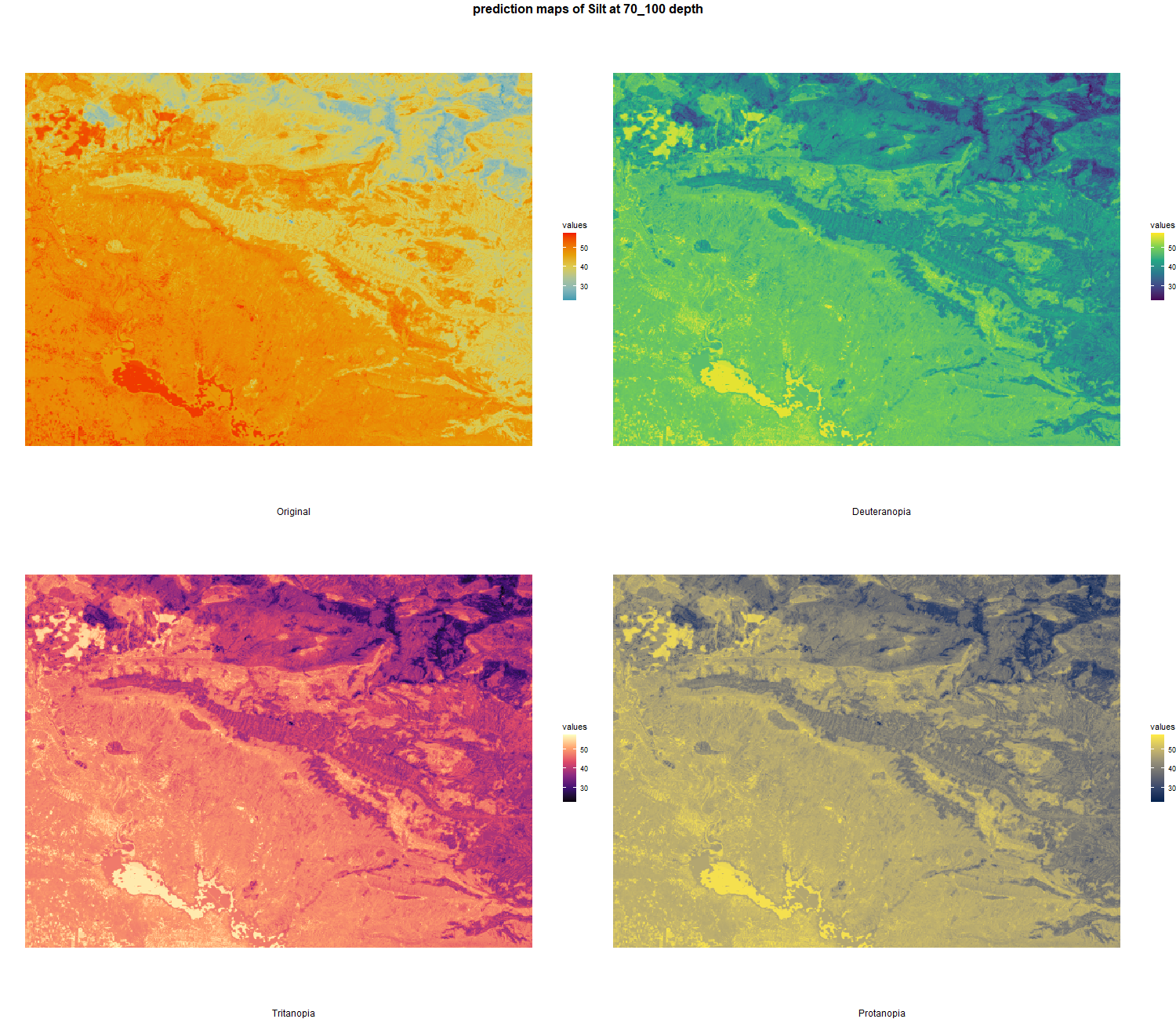
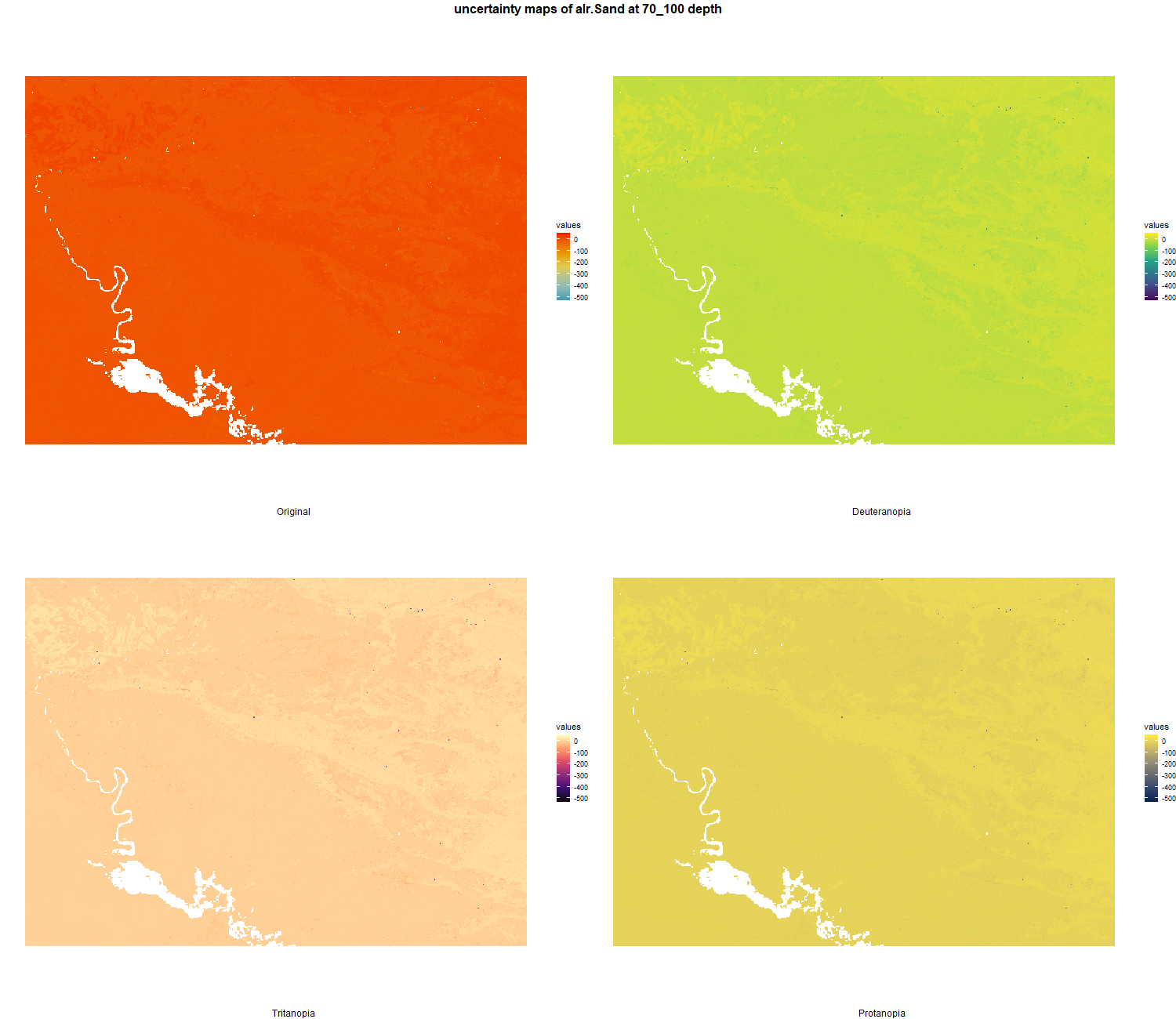
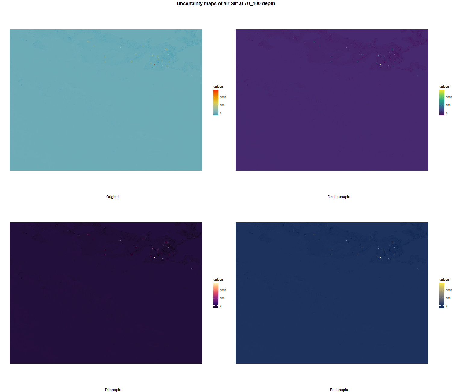
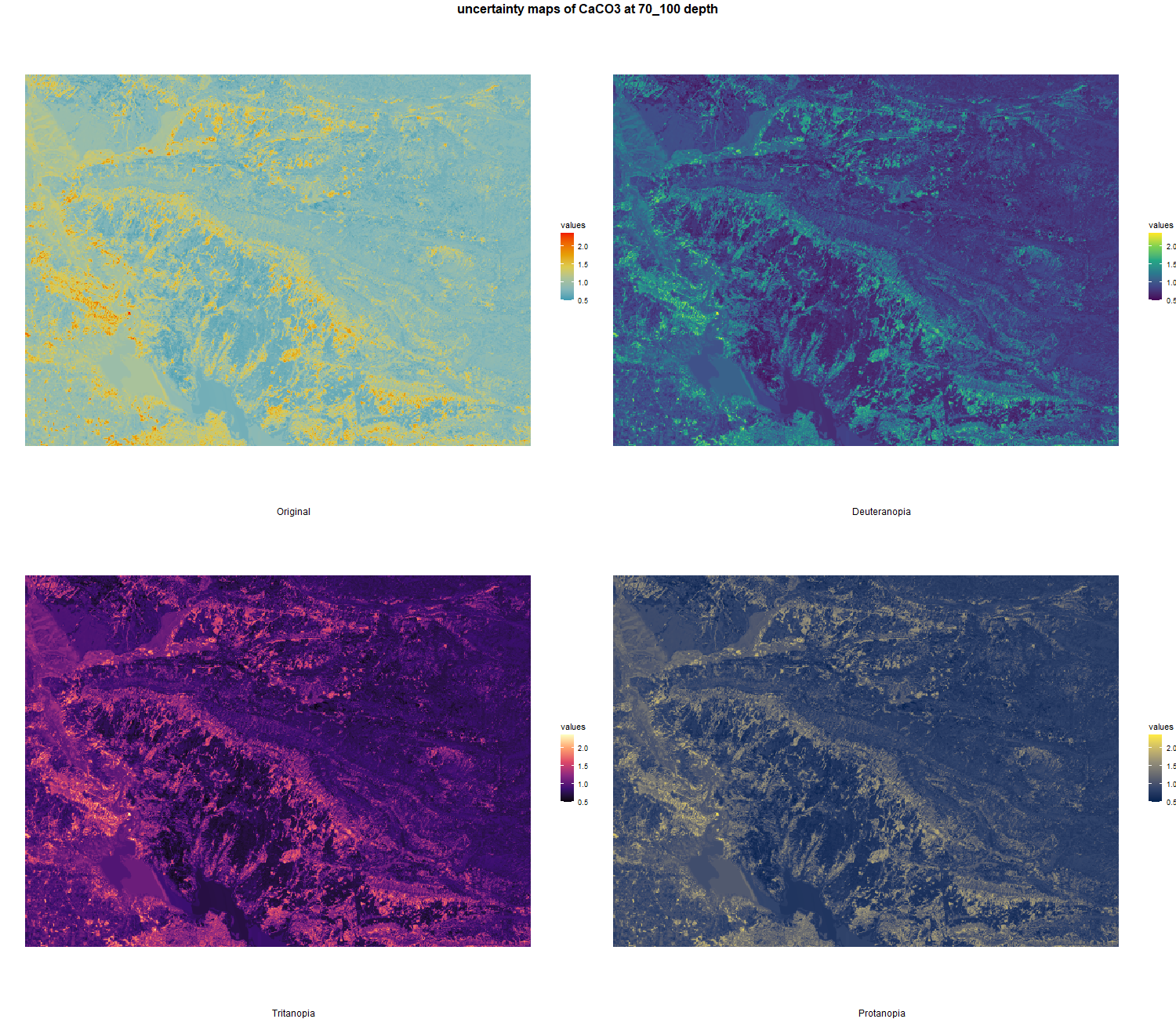
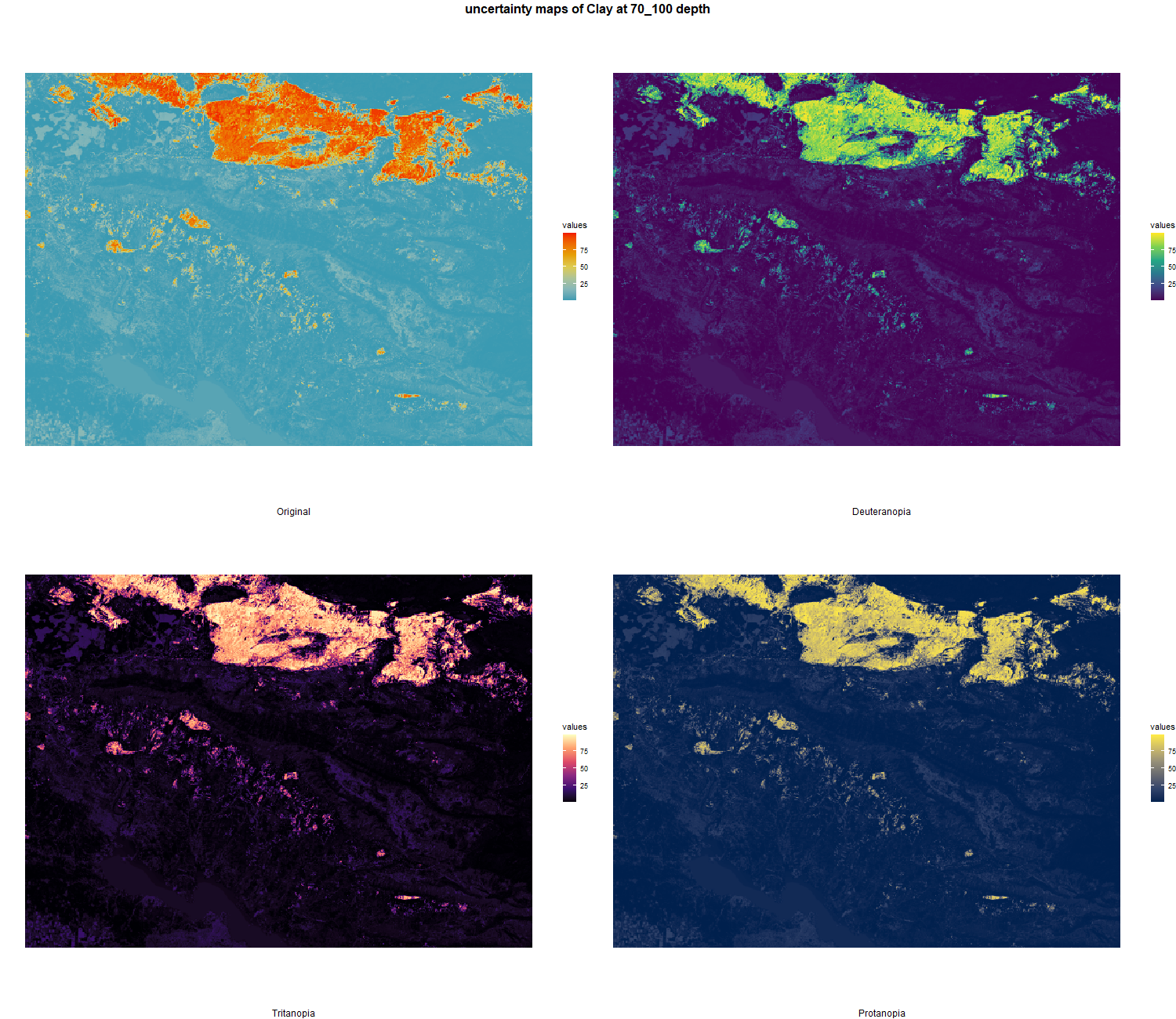
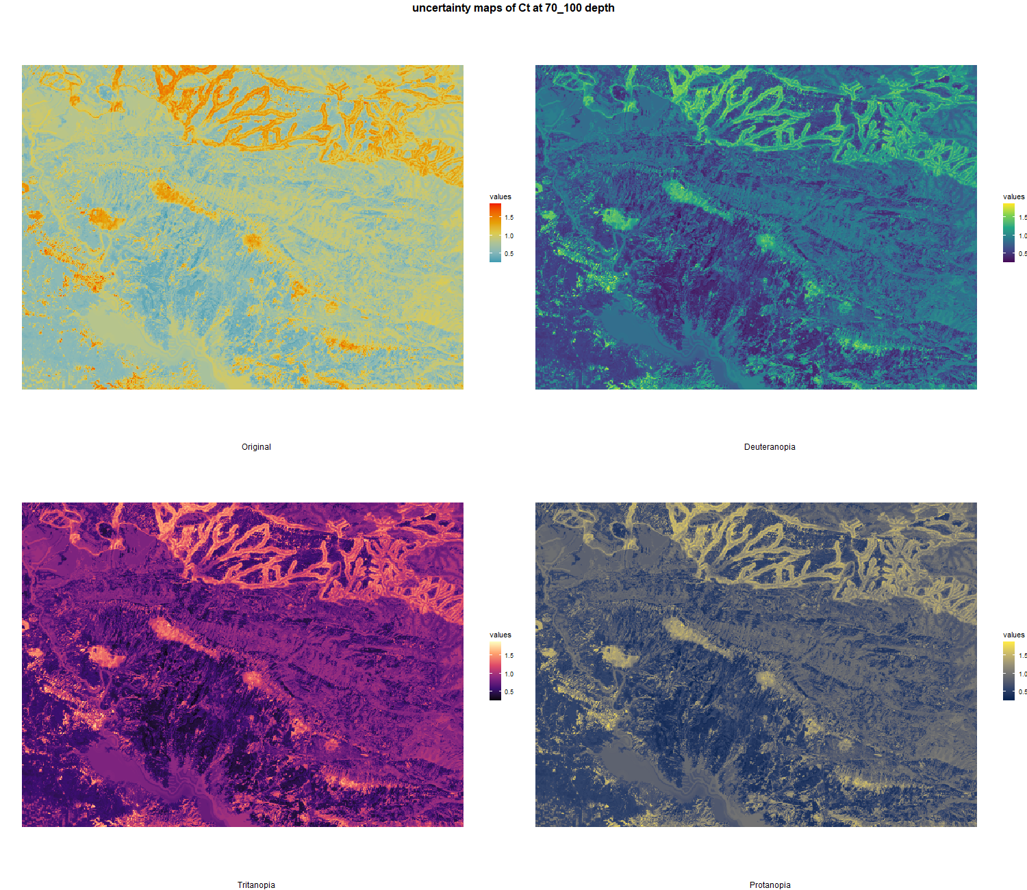
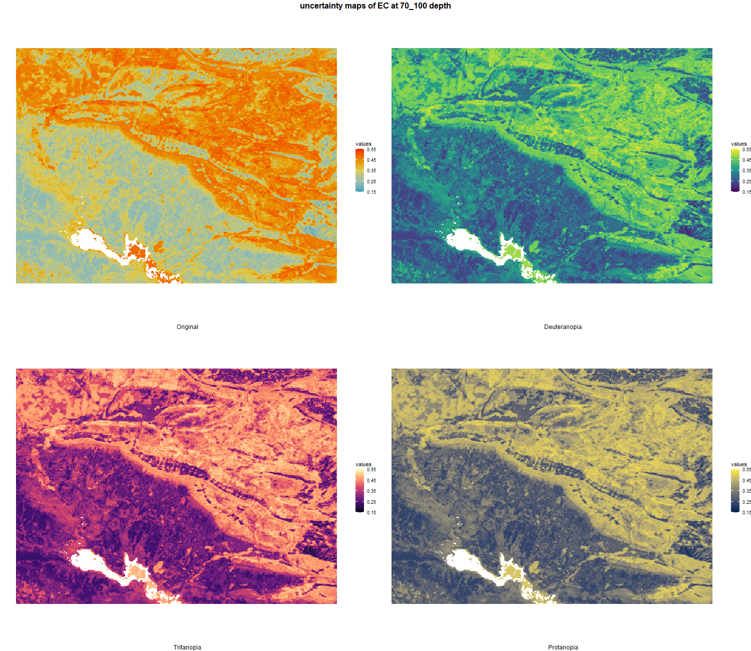
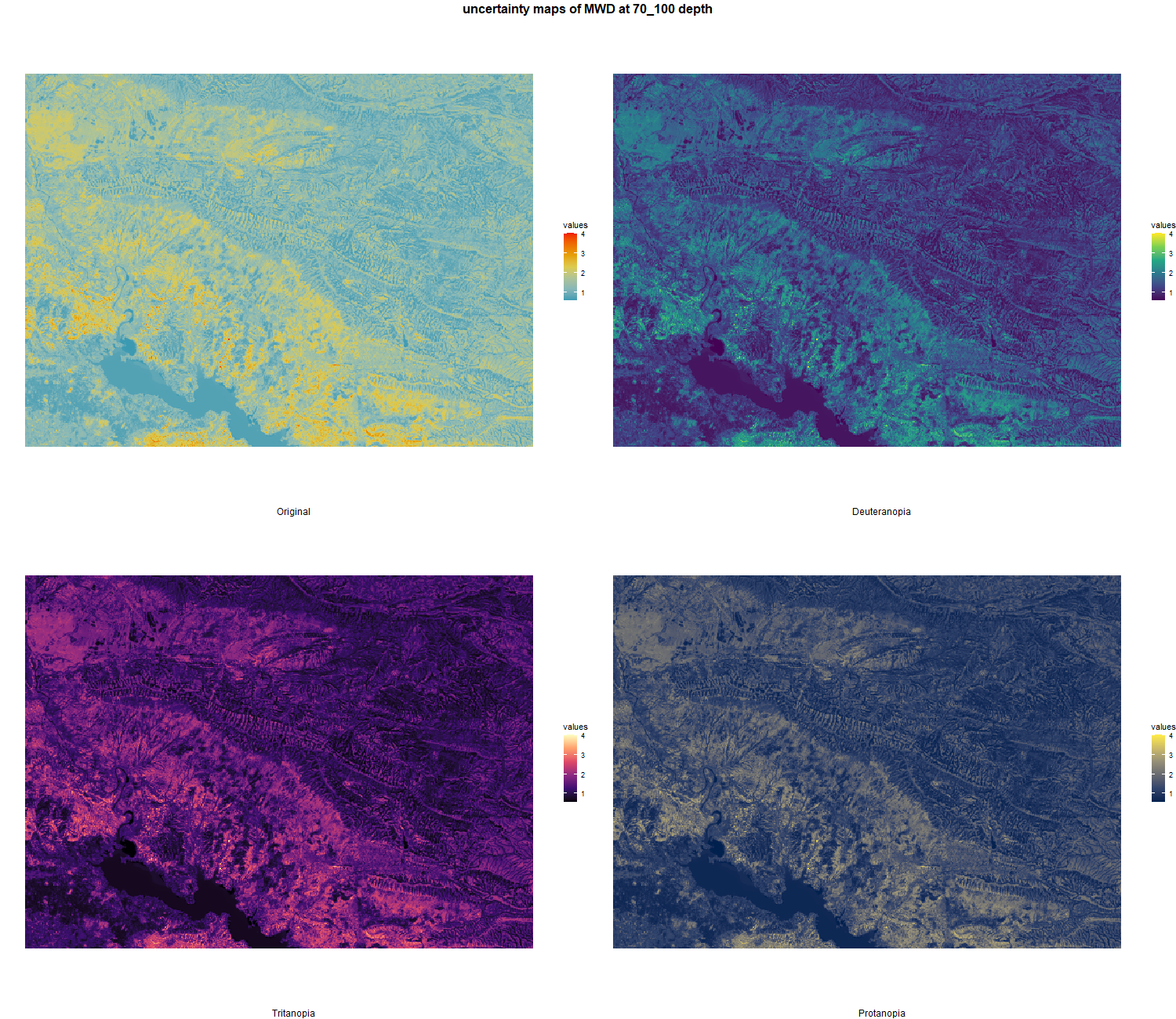
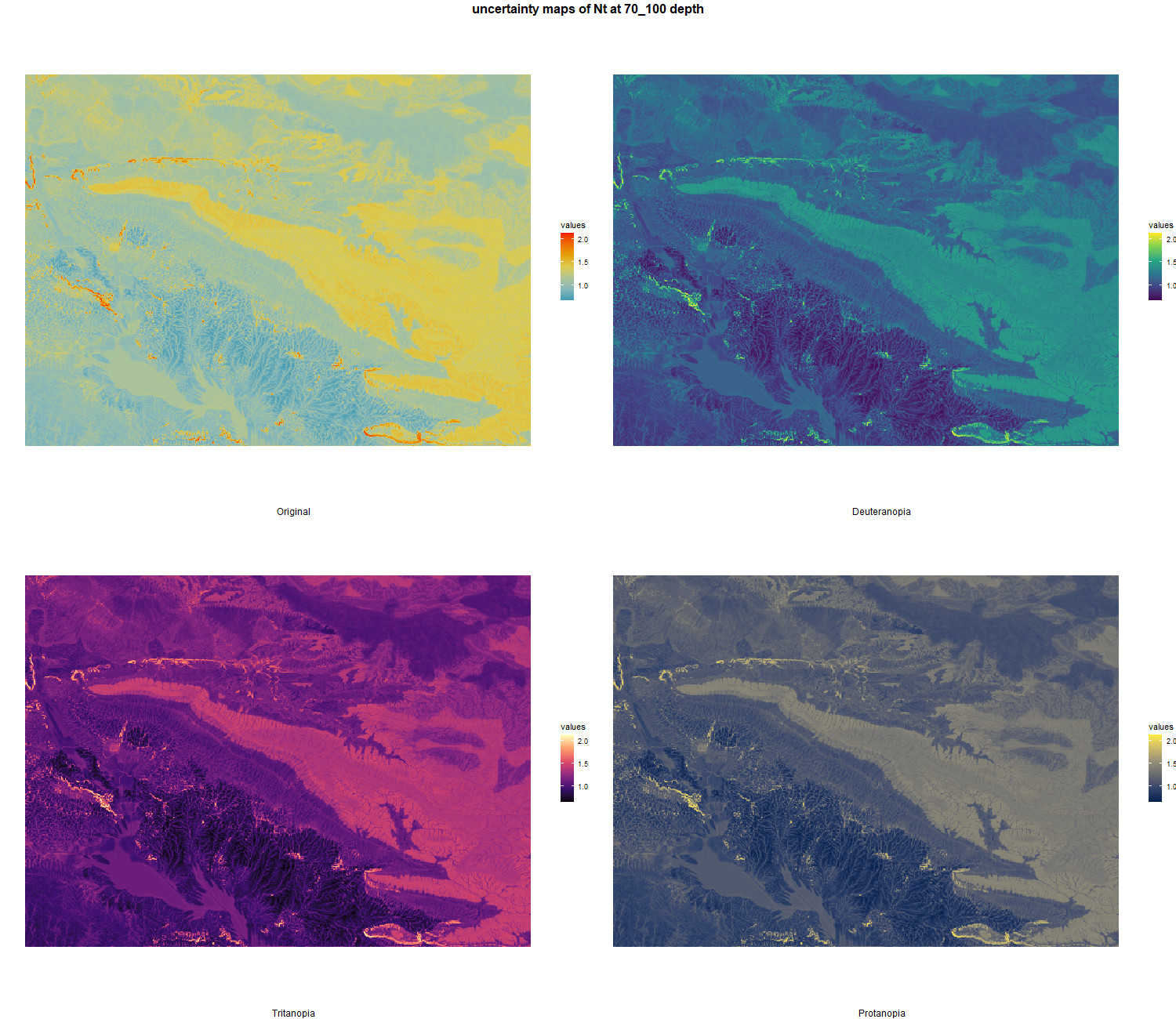
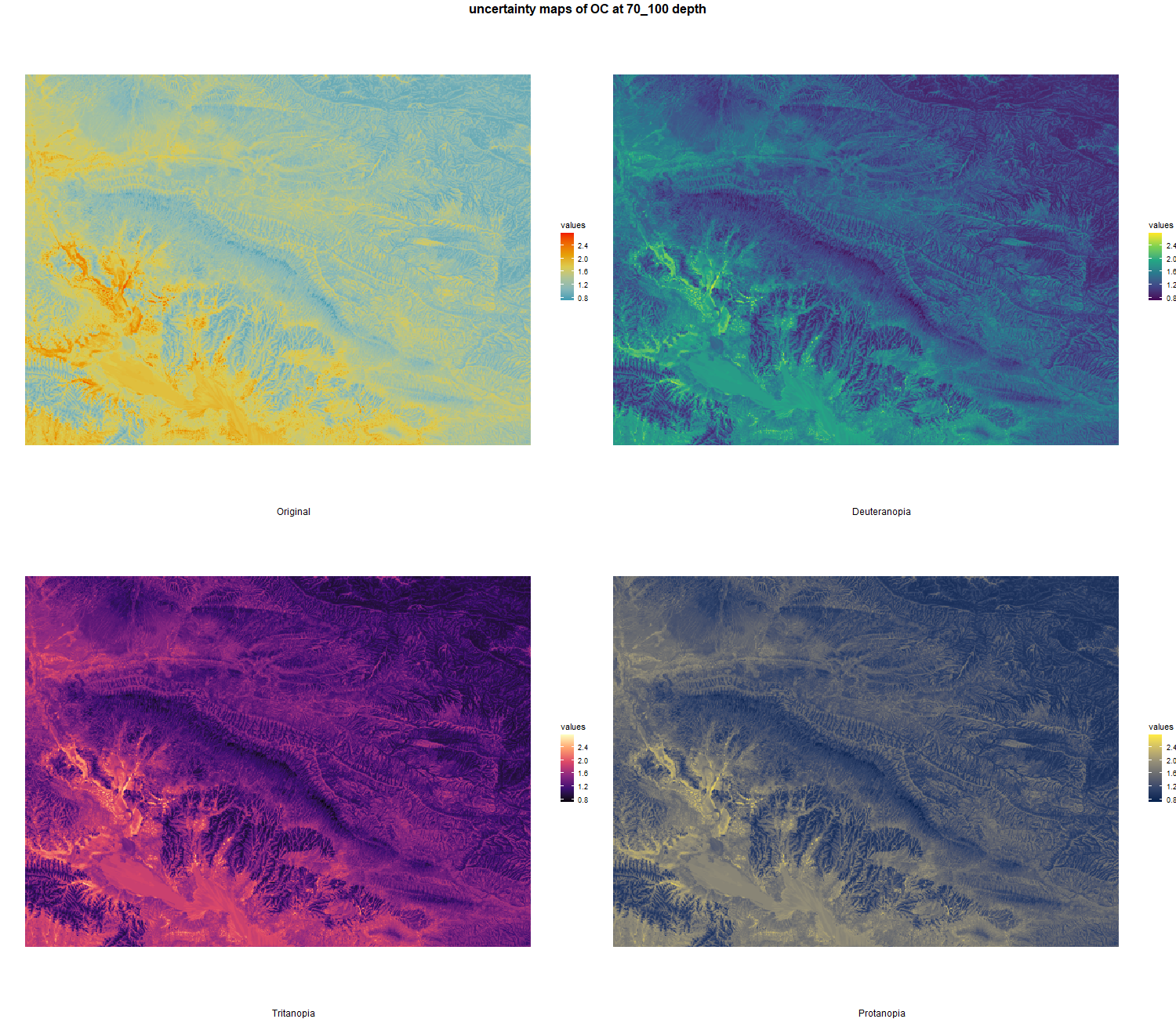
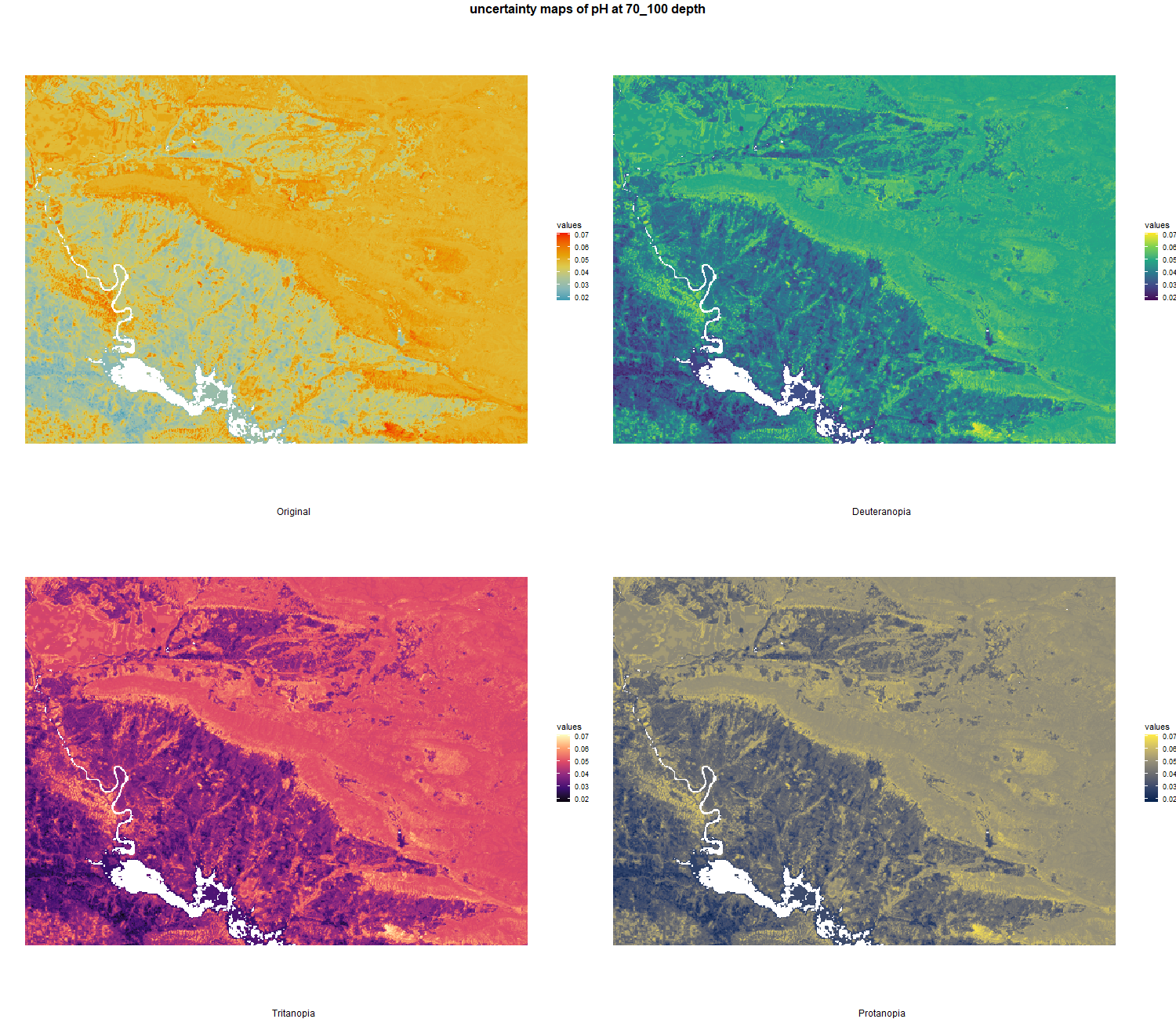
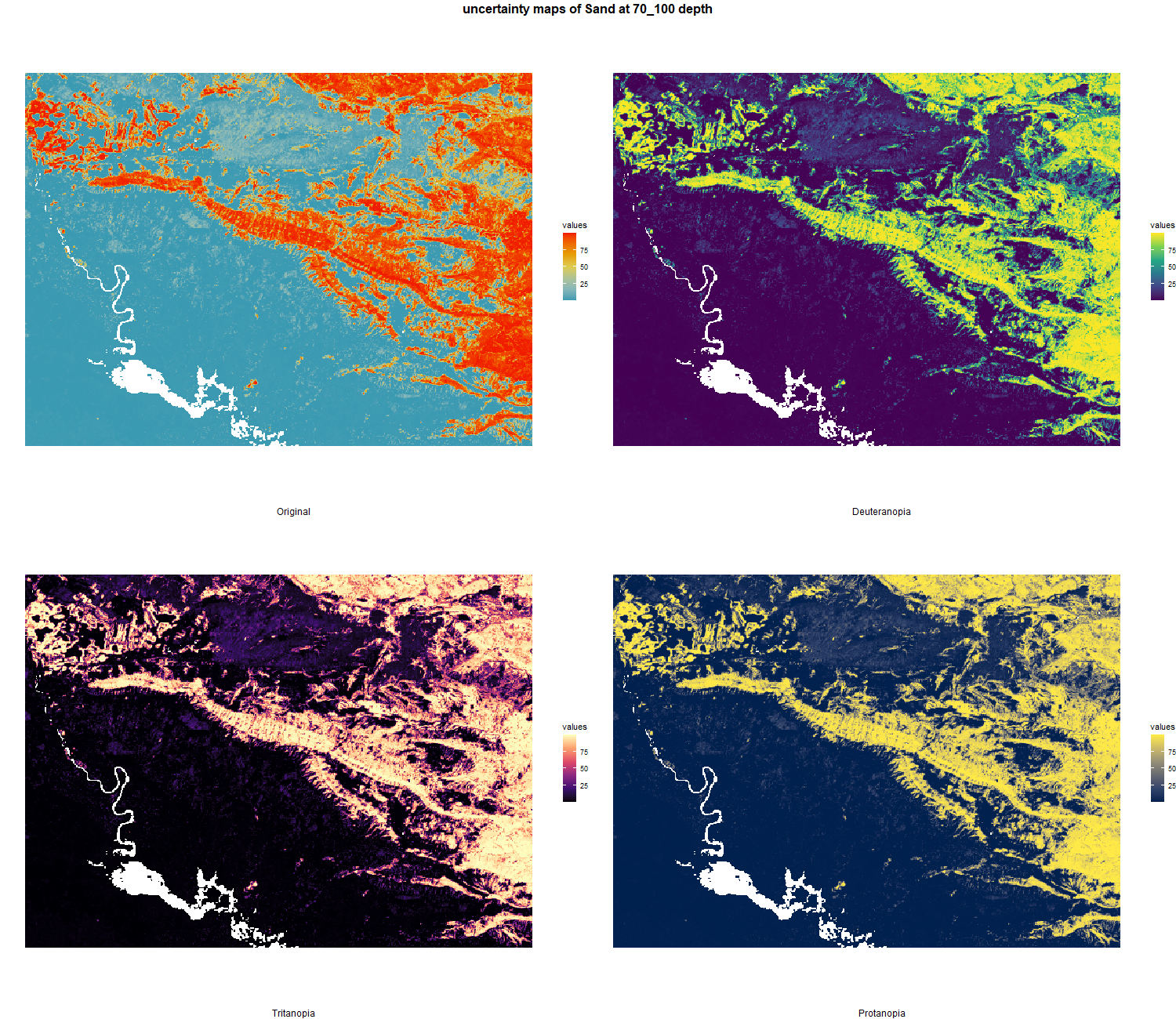
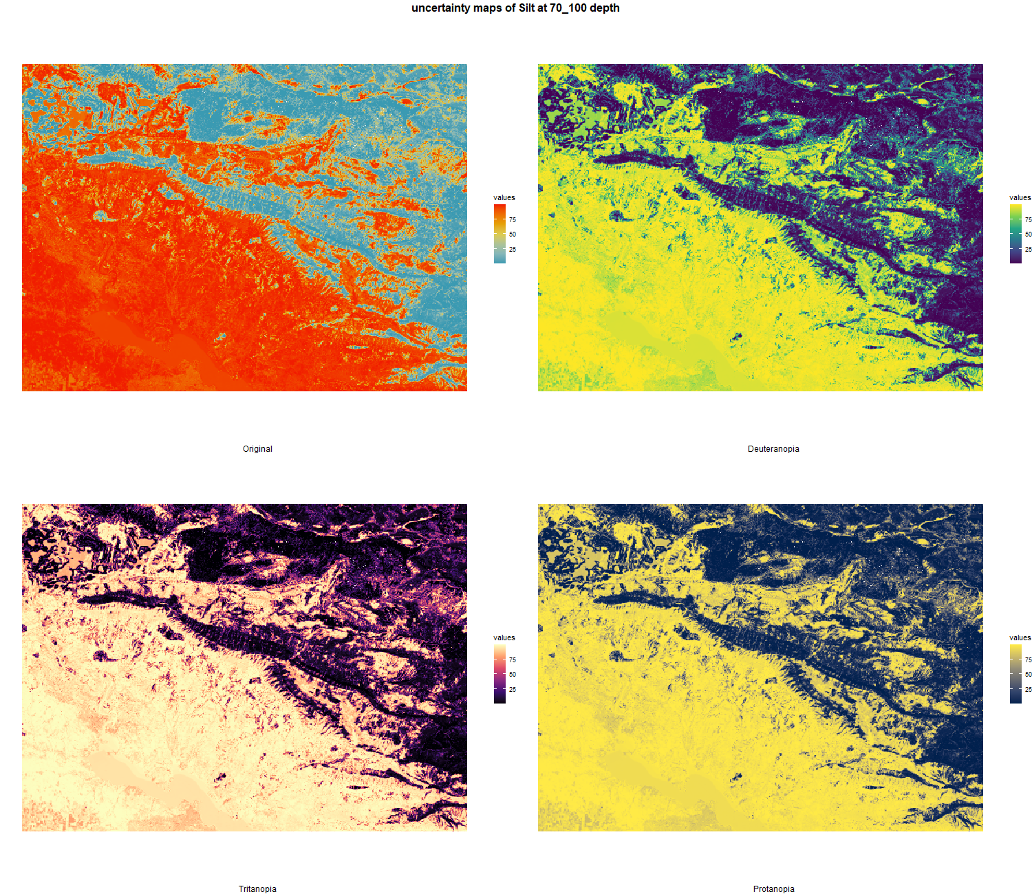
We produced also maps of all properties prediction and uncertainty
 # 08.5 Combined plots of each variables ========================================

    raster_resize_croped <- crop(raster_resize, survey)
    raster_resize_masked <- mask(raster_resize_croped, survey)
    rasterdf <- as.data.frame(raster_resize_masked, xy = TRUE)
    rasterdf <- rasterdf[complete.cases(rasterdf),]

    legend <- c("pH [KCl]", "CaCO3 [%]", "Nt [%]" , "Ct [%]", "OC [%]", "EC [µS/cm-1]", "MWD [mm]", "alr.Sand", "alr.Silt", "Sand [%]", "Silt [%]", "Clay [%]")

    bounds <- st_bbox(survey)
    xlim_new <- c(bounds["xmin"] - 3000, bounds["xmax"] + 3000)
    ylim_new <- c(bounds["ymin"] - 3000, bounds["ymax"] + 3000)

    generate_raster_plot <-    function(rasterdf, value, depth, legend) {
      palette_viridis <- viridis(256)
      t <- value +2
      ggplot() +
        geom_raster(data = rasterdf,
                    aes(x = x, y = y,fill = rasterdf[[t]] )) +
        ggtitle(paste0(type, " map of ", names(rasterdf[t]) , " for ",depth , " cm soil depth")) +
        scale_fill_gradientn(colors = palette_viridis,
                             name = legend) +
        annotation_scale(
          location = "br",
          width_hint = 0.3,
          height = unit(0.3, "cm"),
          line_col = "black",
          text_col = "black",
          bar_cols = c("white", "red")
        ) +
        annotate("text", label = paste("Projection: WGS84 UTM 38N"),
                 x = Inf, y = -Inf, hjust = 1.5, vjust = -3, size = 3, color = "black") +
        annotation_north_arrow(location = "tr", which_north = "true", height = unit(1, "cm"), width = unit(0.75, "cm")) +
        theme_bw() +
        theme(
          panel.grid = element_blank(),
          axis.text.y = element_text(angle = 90, vjust = 0.5, hjust = 0.5),
          axis.title = element_blank(),
          legend.position = "right")+
        coord_equal(ratio = 1)
    }

    stack_graph <- list()

    for (i in 1:nlyr(raster_resize_croped)) {
      stack_graph[[i]] <- generate_raster_plot(rasterdf, i, depth, legend[i])
    }


    png(paste0("./export/visualisations/", depth,"/", type, "_maps_at_",depth,"_depth.png"),    # File name
        width = 2000, height = 1700)

    grid.arrange(grobs = stack_graph, ncol = 3,
                 top = textGrob(paste0(type, " maps at ", depth , " cm depth"), gp = gpar(fontsize = 12, fontface = "bold")))

    dev.off()

    pdf(paste0("./export/visualisations/", depth,"/",type, "_maps_at_",depth,"_depth.pdf"),
        width = 35, height = 30,
        bg = "white",
        colormodel = "cmyk")

    grid.arrange(grobs = stack_graph, ncol = 3,
                 top = textGrob(paste0(type, " maps at ", depth , " cm depth"), gp = gpar(fontsize = 12, fontface = "bold")))

    dev.off()
  }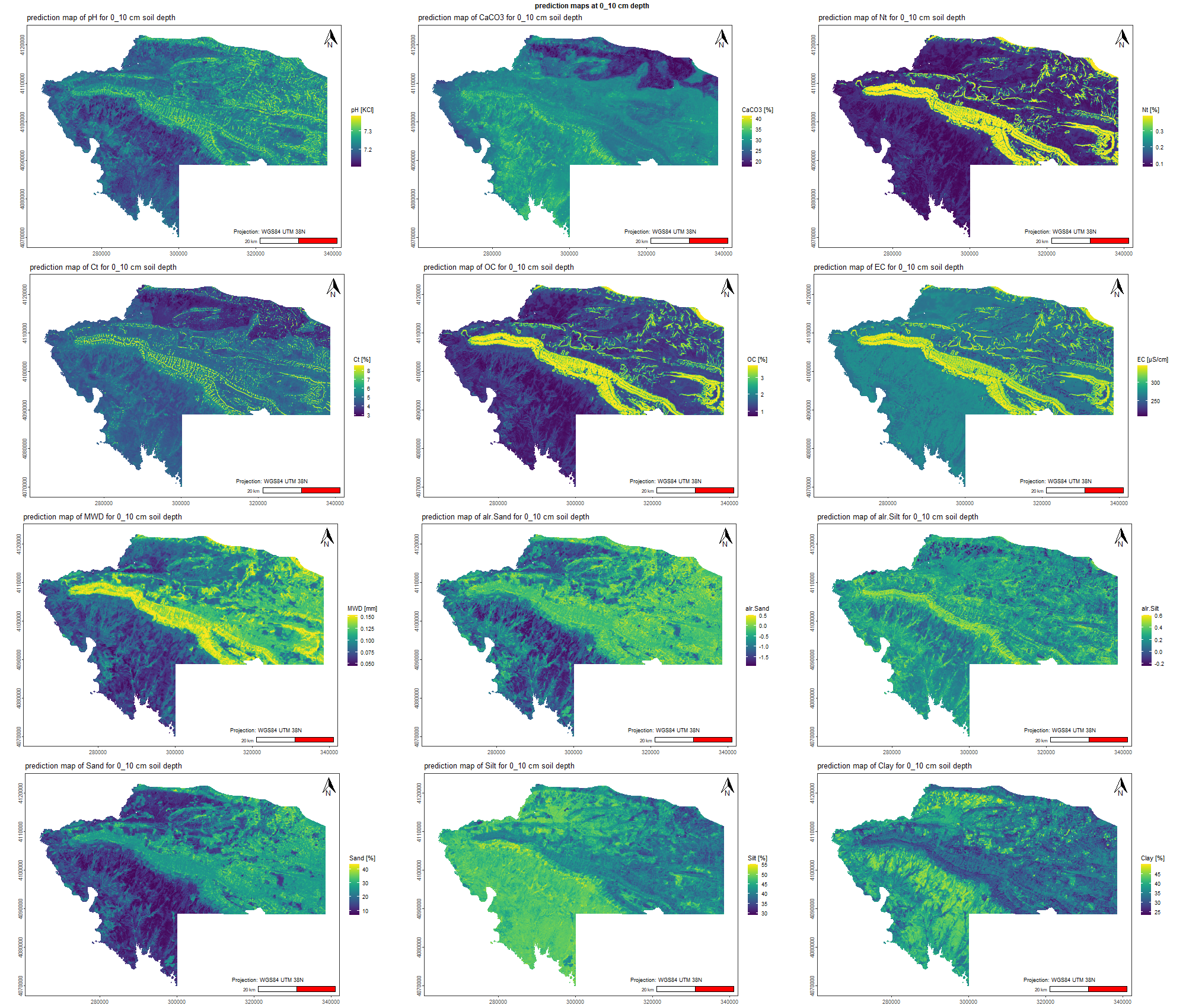
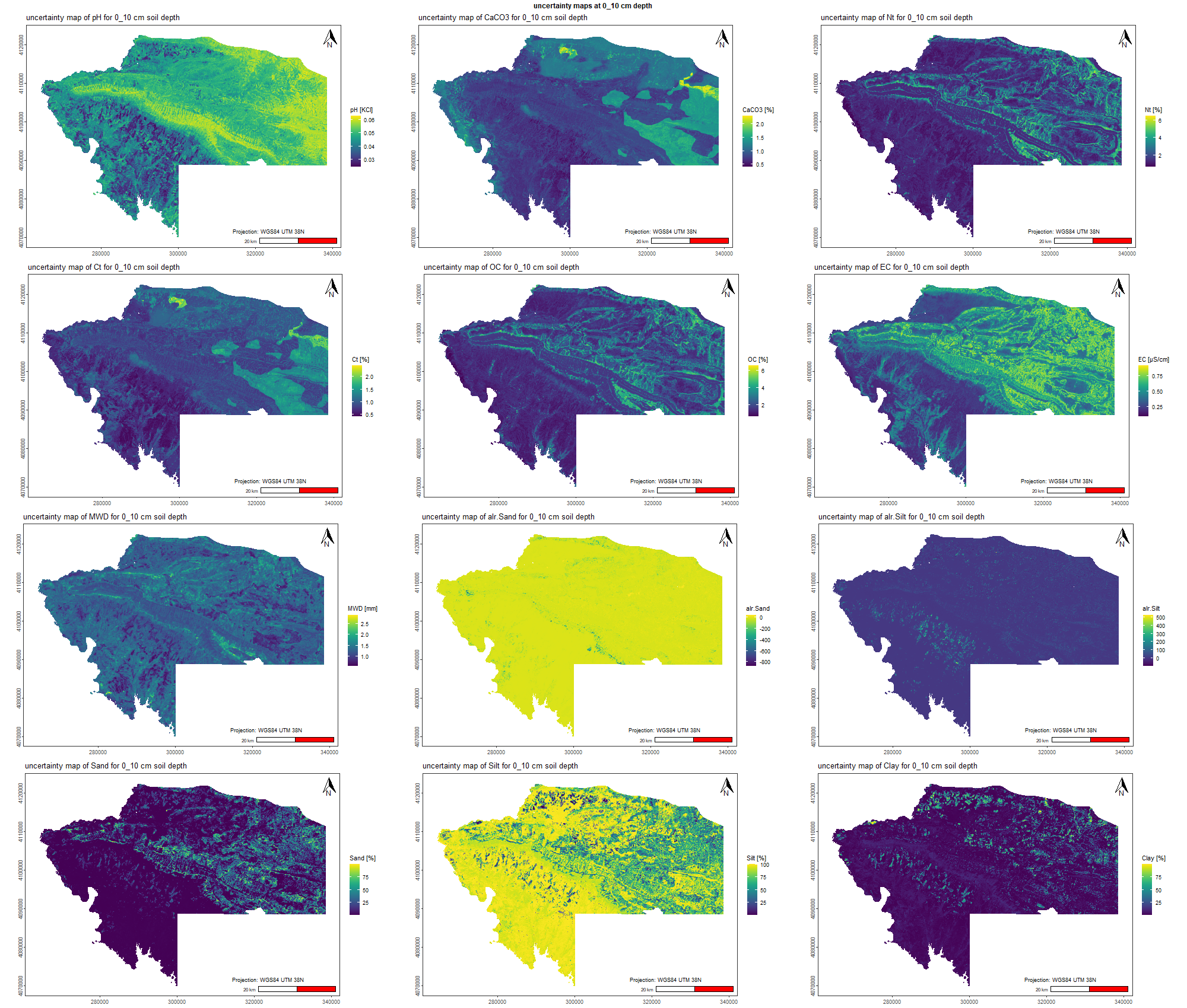
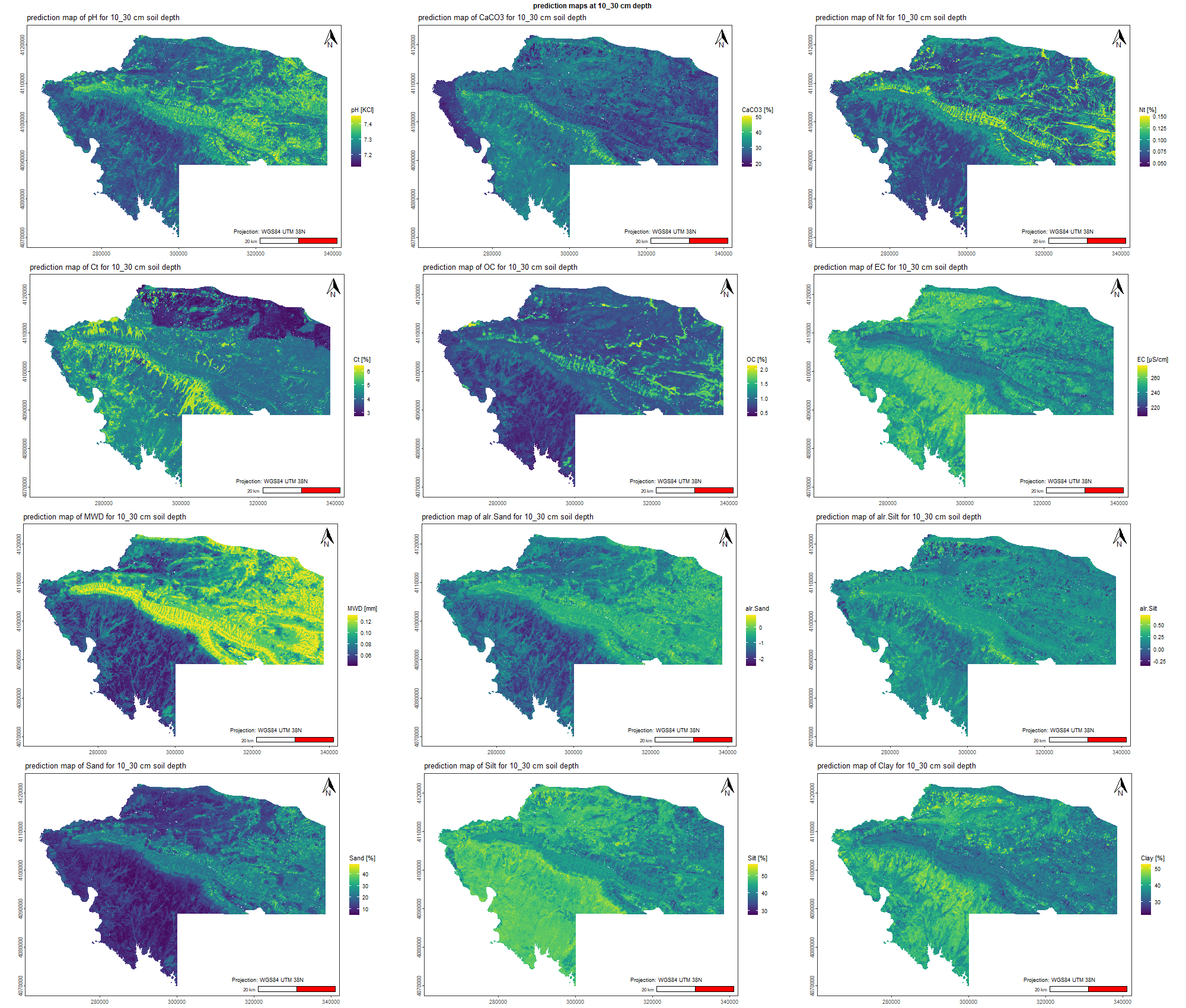
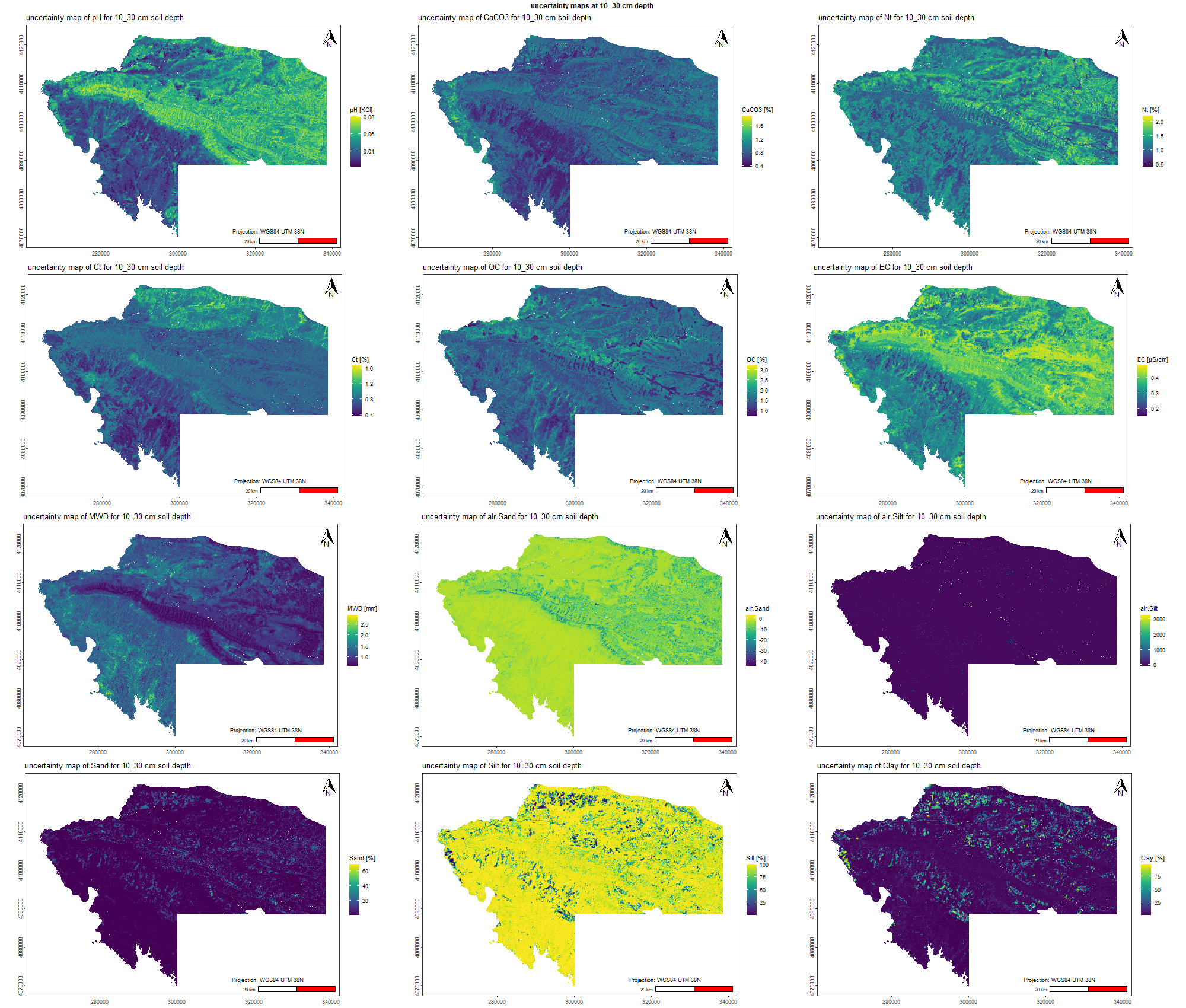
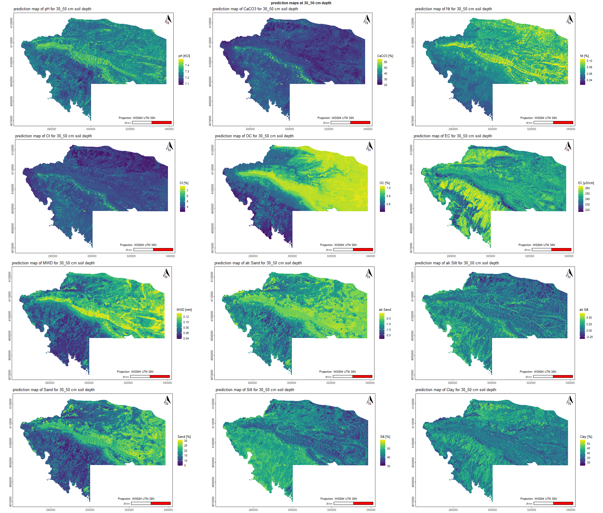
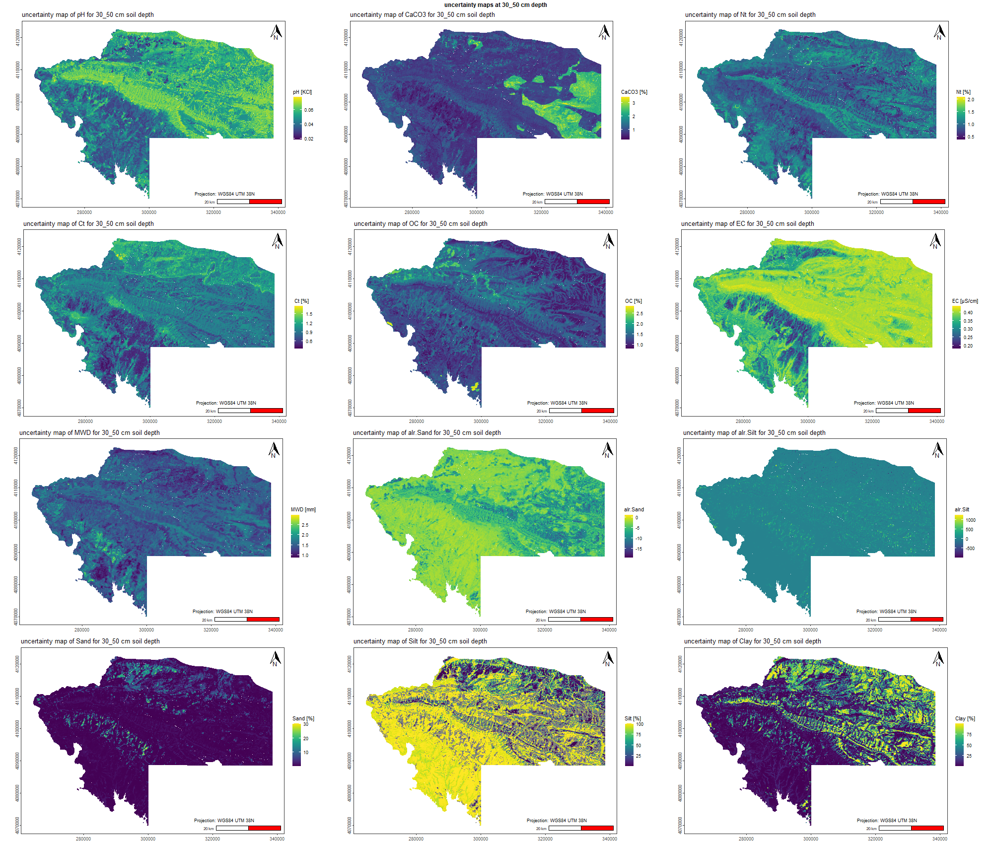
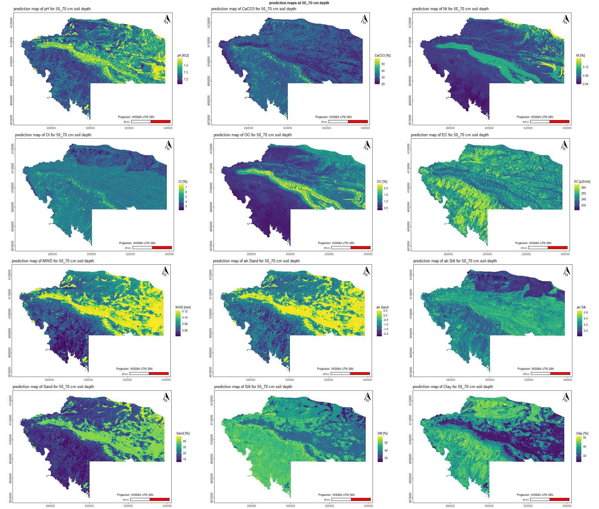
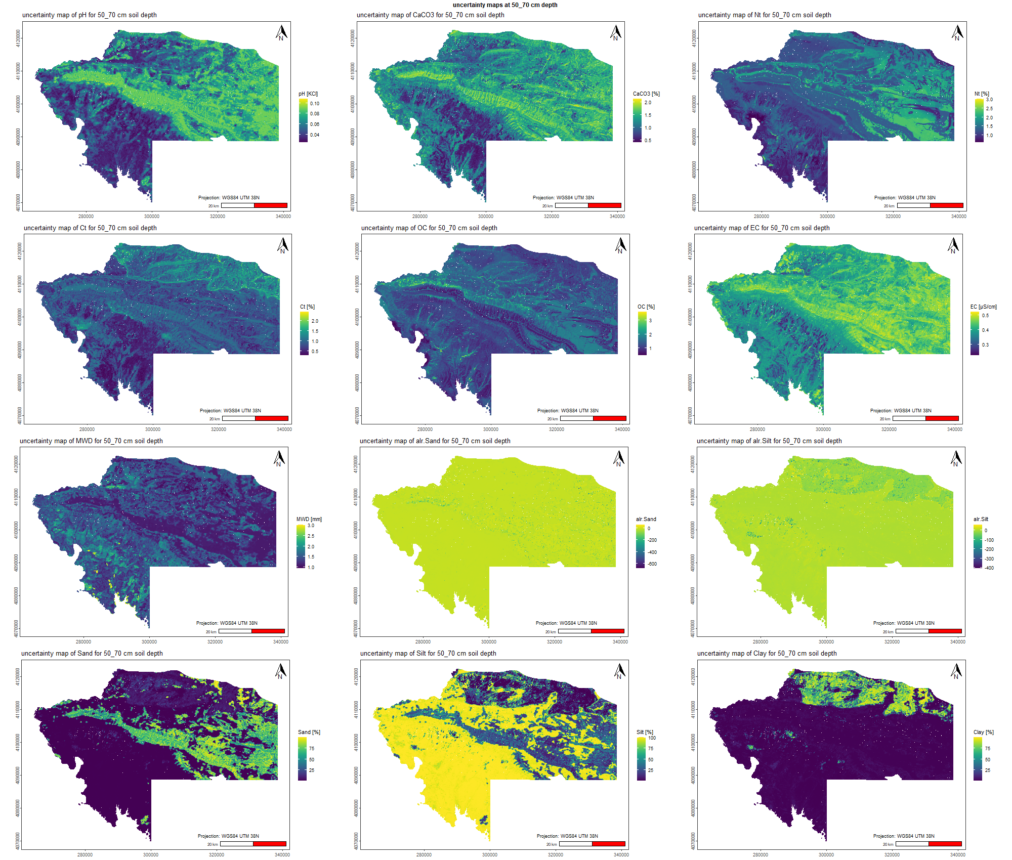
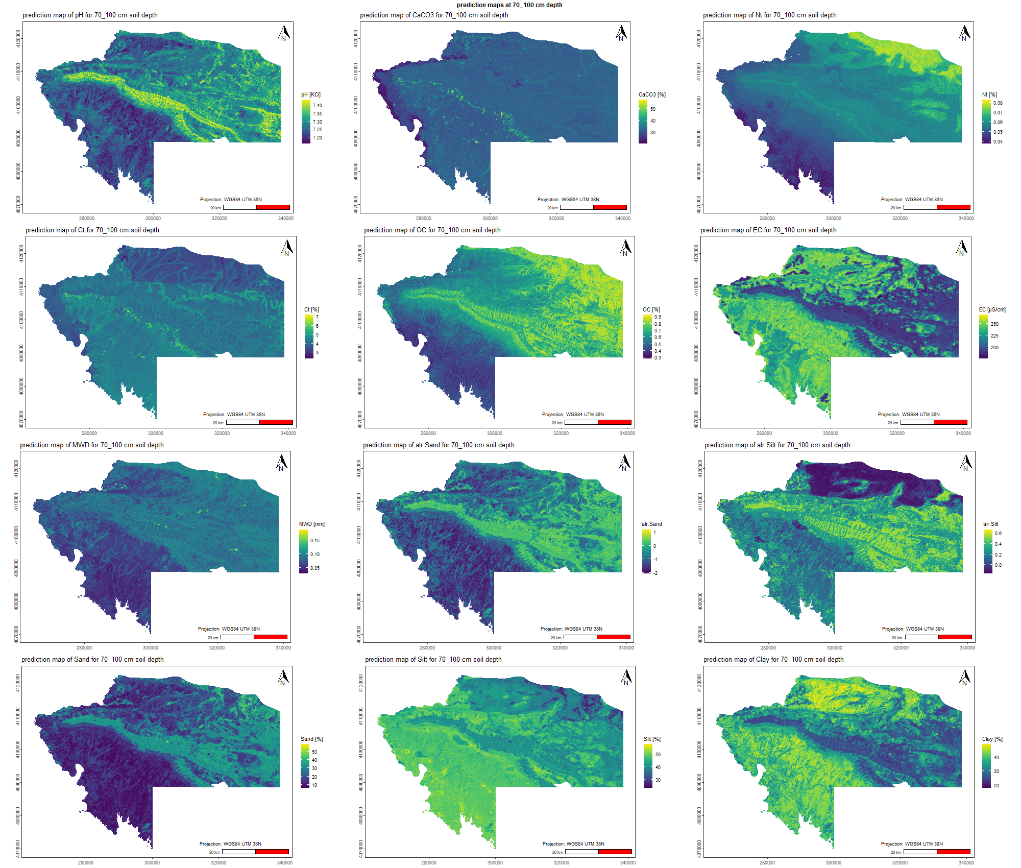
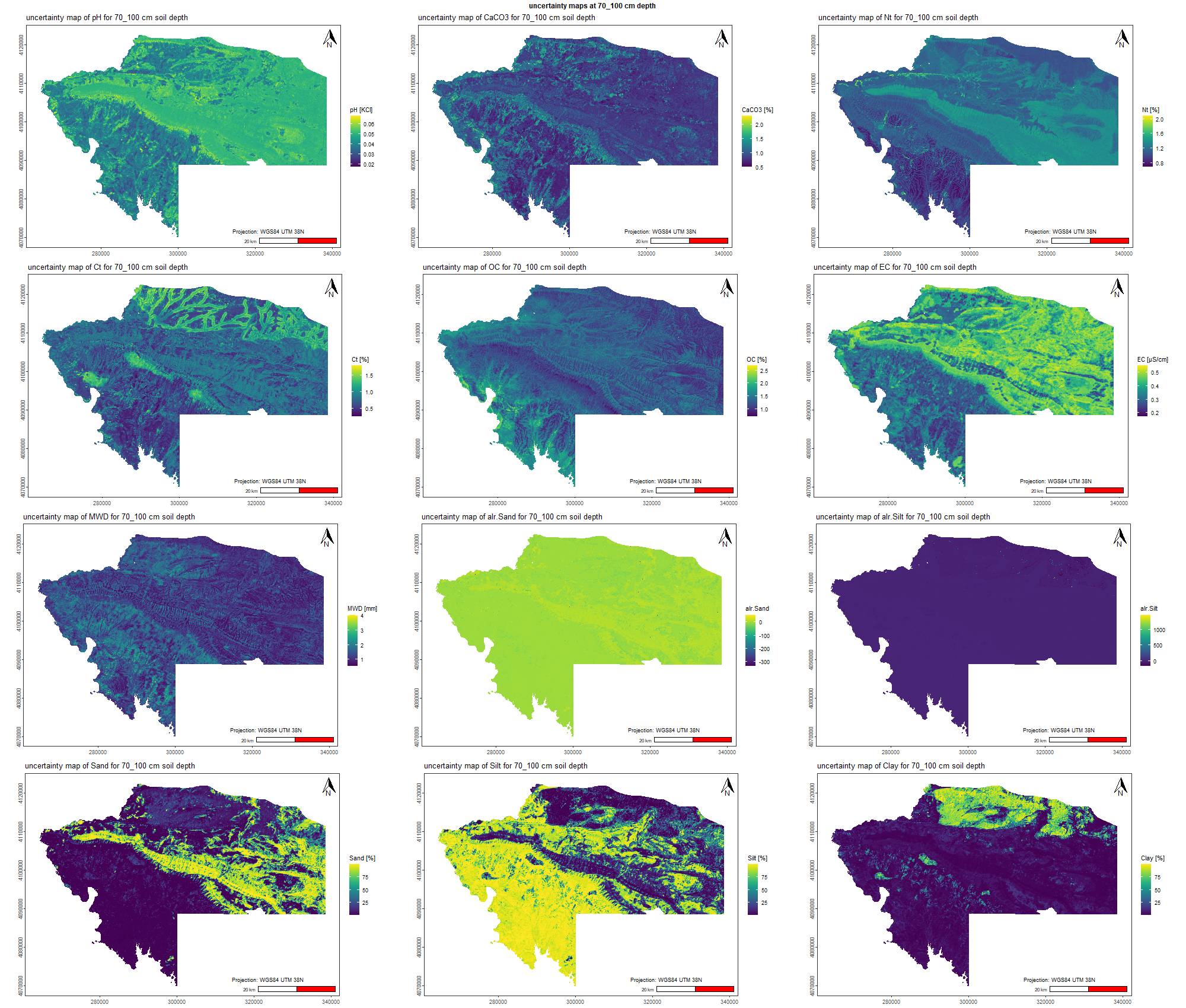
# 08.6 Simplified version for publication =======================================

  raster_resize <- aggregate(raster_stack[[1]], fact=5, fun=mean)
  raster_resize_croped <- crop(raster_resize, survey)
  raster_resize_croped <- focal(raster_resize_croped,
                                w = 3,
                                fun = "mean",
                                na.policy = "only",
                                na.rm = TRUE)
  raster_resize_masked <- mask(raster_resize_croped, survey)
  rasterdf <- as.data.frame(raster_resize_masked, xy = TRUE)
  rasterdf <- rasterdf[complete.cases(rasterdf),]

  generate_clean_raster_plot <- function(rasterdf, i, legend, depth) {
    palette_viridis <- viridis(256)
    t <- i + 2
    p <- ggplot() +
      geom_raster(data = rasterdf, aes(x = x, y = y, fill = rasterdf[[t]])) +
      ggtitle(paste0("Prediction map of ", colnames(rasterdf)[t])) +
      scale_fill_gradientn(colors = palette_viridis, name = legend) +
      theme_void() +
      theme(
        legend.position = "right",
        plot.title = element_text(size = 8),
        legend.title = element_text(size = 6),
        legend.text = element_text(size = 6),
        legend.key.size = unit(0.3, "cm")) +
      coord_equal(ratio = 1)

    return(p)
  }

  light_pred <- list()

  for (i in 1:nlyr(raster_resize_croped)) {
    light_pred[[i]] <- generate_clean_raster_plot(rasterdf, i, legend[i], depth)
  }


  raster_resize <- aggregate(raster_stack[[2]], fact=5, fun=mean)
  raster_resize_croped <- crop(raster_resize, survey)
  raster_resize_croped <- focal(raster_resize_croped,
                                w = 3,
                                fun = "mean",
                                na.policy = "only",
                                na.rm = TRUE)

  raster_resize_masked <- mask(raster_resize_croped, survey)
  rasterdf <- as.data.frame(raster_resize_masked, xy = TRUE)
  rasterdf <- rasterdf[complete.cases(rasterdf),]

  # Some outliers in the uncertainty maps
  rasterdf$alr.Sand[rasterdf$alr.Sand < -50] <- -50
  rasterdf$alr.Silt[rasterdf$alr.Silt > 50] <- 50

  palette_blue <- colorRampPalette(c("lightblue", "blue", "darkblue"))(7)

  generate_clean_raster_plot <- function(rasterdf, i, legend, depth) {
    palette_viridis <- viridis(256)
    t <- i + 2
    p <- ggplot() +
      geom_raster(data = rasterdf, aes(x = x, y = y, fill = rasterdf[[t]])) +
      ggtitle(paste0("Uncertainty map of ", colnames(rasterdf)[t])) +
      scale_fill_gradientn(colors = palette_blue, name = legend) +
      theme_void() +
      theme(
        legend.position = "right",
        plot.title = element_text(size = 8),
        legend.title = element_text(size = 6),
        legend.text = element_text(size = 6),
        legend.key.size = unit(0.3, "cm")) +
      coord_equal(ratio = 1)

    return(p)
  }

  light_uncer <- list()

  for (i in 1:nlyr(raster_resize_croped)) {
    light_uncer[[i]] <- generate_clean_raster_plot(rasterdf, i, legend[i], depth)
  }

  plots_alternated <- c(rbind(light_pred, light_uncer))

  png(paste0("./export/visualisations/", depth,"/Publication_maps_at_",depth,"_depth.png"),    # File name
      width = 2000, height = 2000)

  grid.arrange(grobs = plots_alternated, ncol = 4,
               top = textGrob(paste0("Prediction and uncertainty maps at ", depth , " cm depth"), gp = gpar(fontsize = 10, fontface = "bold")))

  dev.off()

  pdf(paste0("./export/visualisations/", depth,"/Publication_maps_at_",depth,"_depth.pdf"),
      width = 13, height = 13,
      bg = "transparent",
      colormodel = "cmyk")

  grid.arrange(grobs = plots_alternated, ncol = 4,
               top = textGrob(paste0("Prediction and uncertainty maps at ", depth , " cm depth"), gp = gpar(fontsize = 10, fontface = "bold")))

  dev.off()

}

rm(list=setdiff(ls(), c("make_subdir", "increments")))
7.6.3 SoilGrid evaluation and preparation
We choose to compute top, sub and lower soil to evaluate the SoilGrid 2.0 product with our predictions. Our interval were based on top-soil with 0 - 30 cm; sub-soil with 30 - 70 for our own prediction and 30 - 60 cm for the SoilGrid; lower-soil with 70 - 100 cm for our own prediction and 60 - 100 for SoilGrid 2.0 product.
We had to standardised the values of our prediction to compare them with the SoilGrid 2.0 product (Committee 2015).
# 09 Evaluation with SoilGrid  #################################################
# 09.1 Prepare data ============================================================

# For 0-5 cm increment
files <- list.files("./data/Soil_grid/Values/0_5/", pattern = "*tif", full.names = TRUE)
SoilGrid.zero <- rast(files)
SoilGrid.zero <- project(SoilGrid.zero, "EPSG:32638")

# For 5-15 cm increment
files <- list.files("./data/Soil_grid/Values/5_15/", pattern = "*tif", full.names = TRUE)
SoilGrid.five <- rast(files)
SoilGrid.five <- project(SoilGrid.five, "EPSG:32638")

# For 15-30 cm increment
files <- list.files("./data/Soil_grid/Values/15_30/", pattern = "*tif", full.names = TRUE)
SoilGrid.fifteen <- rast(files)
SoilGrid.fifteen <- project(SoilGrid.fifteen, "EPSG:32638")

# For 30-60 cm increment
files <- list.files("./data/Soil_grid/Values/30_60/", pattern = "*tif", full.names = TRUE)
SoilGrid.thirty <- rast(files)
SoilGrid.thirty <- project(SoilGrid.thirty, "EPSG:32638")

# For 60-100 cm increment
files <- list.files("./data/Soil_grid/Values/60_100/", pattern = "*tif", full.names = TRUE)
SoilGrid.sixty <- rast(files)
SoilGrid.sixty <- project(SoilGrid.sixty, "EPSG:32638")

Soil_info <- list("Top_pred" = NA,
                  "Top_SoilGrid" = NA,
                  "Sub_pred" = NA,
                  "Sub_SoilGrid" = NA,
                  "Lower_pred" = NA,
                  "Lower_SoilGrid" = NA)

# 09.2 Extract the test samples for metrics analysis ===========================

load("./export/save/Models_DSM_split_Boruta.RData")

soil_infos <- read.csv("./data/MIR_spectra_prediction.csv", sep=";")
soil_infos$Depth..bot <- as.factor(soil_infos$Depth..bot)
soil_infos <- soil_infos[,-c(5,7,8)]
soil_list <- split(soil_infos, soil_infos$Depth..bot)

names(soil_list) <- increments

soil_infos <- soil_list
for (i in 1:length(soil_infos)) {
  soil_infos[[i]] <- soil_infos[[i]][,-c(2,5)]
  colnames(soil_infos[[i]]) <- c("Site_name","Latitude","Longitude","pH","CaCO3","Nt","Ct","Corg","EC","Sand","Silt","Clay","MWD")
  soil_infos[[i]] <- st_as_sf(soil_infos[[i]], coords = c("Longitude", "Latitude"), crs = 4326)
  soil_infos[[i]] <-st_transform(soil_infos[[i]], crs = 32638)
}


SoilGrid.full <- list(SoilGrid.zero, SoilGrid.five, SoilGrid.fifteen, SoilGrid.thirty, SoilGrid.sixty)
names(SoilGrid.full) <- increments

Stats_final <- list()

for (depth in increments) {
  test_rows <- row.names(Models[[depth]]$Test_data[[1]])
  soil_test <- soil_infos[[depth]][row.names(soil_infos[[depth]]) %in% test_rows, ]
  Soil.Grid_df <- terra::extract(SoilGrid.full[[depth]], soil_test)

  # Convert to % values and reduce the pH by 10 to fit our values
  Soil.Grid_df <- Soil.Grid_df[,-1]
  colnames(Soil.Grid_df) <- c("Clay", "OC", "Nt", "pH", "Sand", "Silt")
  Soil.Grid_df[,c(1,4:6)] <- Soil.Grid_df[,c(1,4:6)]/10

  # pH standardisation Aitken and Moody (1991) R2 =  0.78
  Soil.Grid_df[4] <- (1.28 * Soil.Grid_df[4])  - 0.613

  Soil.Grid_df[2] <- Soil.Grid_df[2]/1000
  Soil.Grid_df[3] <- Soil.Grid_df[3]/10000

  sum(Soil.Grid_df == 0)
  summary(Soil.Grid_df[1:6])

  layers <- c(1,3,5,8,9)
  preds <- data.frame(NULL)
  for (j in layers) {
   data <- Models[[depth]]$Test_data[[j]]
   data <- data[,c(1:length(data)-1)]
   values <- predict(Models[[depth]]$Models[[j]]$finalModel, newdata = data, what = 0.5)
   ifelse(nrow(preds) == 0, preds <- as.data.frame(values), preds <- cbind(preds, values))
  }

  y <- preds[,c(4:5)]
  alr_pred <- as.data.frame(alrInv(y))
  preds[,c(4:6)] <- 100*(alr_pred)
  colnames(preds) <- c("pH", "Nt", "OC", "Sand", "Silt", "Clay")

  # pH standardisation Aitken and Moody (1991) R2 = 0.8
  preds[1] <- (1.175*preds[1]) - 0.262

  # Texture standardisation Minasny and McBratney (2001) 0.063 to 0.05

  Texture <- preds[,c(4:6)]
  colnames(Texture) <- c("SAND","SILT", "CLAY")
  Texture <- TT.normalise.sum(Texture, css.names =  c("SAND","SILT", "CLAY"))

  Texture <- TT.text.transf(
    tri.data = Texture, dat.css.ps.lim = c(0, 0.002, 0.063, 2),  # German system
    base.css.ps.lim = c(0, 0.002, 0.05, 2) # USDA system
  )

  preds[,c(4:6)] <- Texture

  # Ground truth control
  obs <- st_drop_geometry(soil_test[,c(2,4,6,8:10)])
  colnames(obs) <- c("pH", "Nt", "OC", "Sand", "Silt", "Clay")

  # pH standardisation Aitken and Moody (1991) R2 = 0.8
  obs[1] <- (1.175*obs[1]) - 0.262

  # Texture standardisation Minasny and McBratney (2001) 0.063 to 0.05

  Texture <- obs[,c(4:6)]
  colnames(Texture) <- c("SAND","SILT", "CLAY")
  Texture <- TT.normalise.sum(Texture, css.names =  c("SAND","SILT", "CLAY"))

  Texture <- TT.text.transf(
    tri.data = Texture, dat.css.ps.lim = c(0, 0.002, 0.063, 2),  # German system
    base.css.ps.lim = c(0, 0.002, 0.05, 2) # USDA system
  )

  obs[,c(4:6)] <- Texture

  Soil.Grid_df <- Soil.Grid_df[, colnames(obs)]
  soil_vars <- colnames(obs)
  stats <- data.frame()

  for (var in soil_vars) {
    true <- obs[[var]]
    Soil.grid.pred <- Soil.Grid_df[[var]]
    Model.pred <- preds[[var]]

    metric <- c("ME", "RMSE", "R2")
    ME  <- mean(Soil.grid.pred - true, na.rm = TRUE)
    RMSE <- sqrt(mean((Soil.grid.pred - true)^2, na.rm = TRUE))
    R2   <- cor(Soil.grid.pred, true, use = "complete.obs")^2

    value <- c(ME, RMSE, R2)
    for (k in 1:3) {
      line.1 <- c(var, depth, "Soil.Grid", metric[k], value[k])
      ifelse(ncol(stats) == 0, stats <- as.data.frame(t(line.1)) , stats <- rbind(stats, line.1))
    }

    ME  <- mean(Model.pred - true, na.rm = TRUE)
    RMSE <- sqrt(mean((Model.pred - true)^2, na.rm = TRUE))
    R2   <- cor(Model.pred, true, use = "complete.obs")^2

    value <- c(ME, RMSE, R2)
    for (k in 1:3) {
      line.2 <- c(var, depth, "Model", metric[k], value[k])
      stats <- rbind(stats, line.2)
    }
  }

  Stats_final[[depth]] <- stats
}

final_table <- do.call(rbind, Stats_final)
colnames(final_table) <- c("Variable", "Depth", "Model", "Metric", "Value")
final_table$Value <- as.numeric(final_table$Value)
write.csv2(final_table, "./export/evaluation/Final_metrics_SoilGrids.csv")

final_metrics <- final_table %>%
  mutate(Value = round(Value, 2)) %>%
  mutate(col = paste(Model, Depth, sep="_")) %>%
  pivot_wider(
    id_cols = c(Variable, Metric),
    names_from = col,
    values_from = Value
  ) %>%
  arrange(Variable, Metric)


df_placement <- final_metrics[3:12]
final_metrics <- cbind(final_metrics[1:2], df_placement[,c(2,1,4,3,6,5,8,7,10,9)])

# Change the "html" to "latex"
kable(final_metrics, "html", escape = FALSE) %>%
  kable_styling(full_width = FALSE) %>%
scroll_box(width = "100%")| Variable | Metric | Model_0_10 | Soil.Grid_0_10 | Model_10_30 | Soil.Grid_10_30 | Model_30_50 | Soil.Grid_30_50 | Model_50_70 | Soil.Grid_50_70 | Model_70_100 | Soil.Grid_70_100 |
|---|---|---|---|---|---|---|---|---|---|---|---|
| Clay | ME | 1.70 | 3.63 | 3.25 | 4.02 | 0.71 | 4.86 | -1.29 | 3.18 | 1.07 | 4.87 |
| Clay | R2 | 0.28 | 0.00 | 0.45 | 0.03 | 0.24 | 0.00 | 0.23 | 0.05 | 0.48 | 0.03 |
| Clay | RMSE | 6.48 | 8.36 | 8.08 | 12.26 | 7.14 | 9.72 | 8.14 | 9.12 | 7.08 | 14.25 |
| Nt | ME | -0.02 | -0.10 | 0.00 | -0.05 | 0.00 | -0.04 | -0.01 | -0.05 | 0.00 | -0.03 |
| Nt | R2 | 0.64 | 0.13 | 0.23 | 0.01 | 0.14 | 0.03 | 0.22 | 0.01 | 0.08 | 0.03 |
| Nt | RMSE | 0.05 | 0.12 | 0.02 | 0.05 | 0.02 | 0.04 | 0.04 | 0.06 | 0.02 | 0.04 |
| OC | ME | -0.24 | -1.18 | -0.11 | -0.69 | -0.08 | -0.60 | -0.07 | -0.60 | 0.02 | -0.51 |
| OC | R2 | 0.46 | 0.10 | 0.68 | 0.03 | 0.15 | 0.00 | 0.76 | 0.08 | 0.30 | 0.00 |
| OC | RMSE | 0.61 | 1.39 | 0.27 | 0.77 | 0.30 | 0.68 | 0.34 | 0.76 | 0.17 | 0.55 |
| Sand | ME | -2.60 | -2.23 | -3.90 | -2.83 | -1.78 | -1.82 | 0.23 | -1.11 | -2.96 | -6.33 |
| Sand | R2 | 0.29 | 0.00 | 0.55 | 0.11 | 0.01 | 0.00 | 0.51 | 0.02 | 0.51 | 0.01 |
| Sand | RMSE | 8.43 | 9.84 | 10.12 | 13.91 | 9.36 | 8.85 | 8.69 | 12.80 | 8.97 | 14.50 |
| Silt | ME | 0.90 | -1.56 | 0.65 | -3.28 | 1.07 | -3.05 | 1.06 | -3.30 | 1.89 | -4.79 |
| Silt | R2 | 0.17 | 0.07 | 0.30 | 0.03 | 0.04 | 0.12 | 0.55 | 0.21 | 0.39 | 0.10 |
| Silt | RMSE | 5.10 | 5.52 | 5.10 | 8.37 | 6.27 | 6.33 | 4.45 | 8.34 | 5.31 | 13.88 |
| pH | ME | 0.02 | 0.46 | -0.02 | 0.28 | 0.03 | 0.51 | 0.05 | 0.35 | 0.01 | -0.05 |
| pH | R2 | 0.22 | 0.01 | 0.55 | 0.01 | 0.16 | 0.02 | 0.09 | 0.05 | 0.30 | 0.00 |
| pH | RMSE | 0.09 | 0.49 | 0.09 | 0.94 | 0.11 | 0.55 | 0.18 | 0.57 | 0.11 | 2.27 |
# 09.3 Top soil preparation ====================================================

Prediction.zero <- rast("./export/final_maps/0_10_prediction_map.tif")
Prediction.zero <- Prediction.zero[[c(1:7,10:12)]]
Prediction.zero<- project(Prediction.zero, "EPSG:32638")
Prediction.ten <- rast("./export/final_maps/10_30_prediction_map.tif")
Prediction.ten <- Prediction.ten[[c(1:7,10:12)]]
Prediction.ten <- project(Prediction.ten, "EPSG:32638")

# Resize and resample
SoilGrid.zero_crop <- crop(SoilGrid.zero, Prediction.zero$pH)
SoilGrid.five_crop <- crop(SoilGrid.five, Prediction.zero$pH)
SoilGrid.fifteen_crop <- crop(SoilGrid.fifteen, Prediction.zero$pH)

Prediction.zero_resample <- resample(Prediction.zero, SoilGrid.zero_crop, method = "bilinear")
Prediction.ten_resample <- resample(Prediction.ten, SoilGrid.zero_crop, method = "bilinear")

# Convert into DF
Prediction.zero_df <- as.data.frame(Prediction.zero_resample, xy = TRUE)
Prediction.zero_df <- Prediction.zero_df[complete.cases(Prediction.zero_df),]

Prediction.ten_df <- as.data.frame(Prediction.ten_resample, xy = TRUE)
Prediction.ten_df <- Prediction.ten_df[complete.cases(Prediction.ten_df),]

SoilGrid.zero_df <- as.data.frame(SoilGrid.zero_crop, xy = TRUE)
SoilGrid.zero_df <- SoilGrid.zero_df[complete.cases(SoilGrid.zero_df),]

SoilGrid.five_df <- as.data.frame(SoilGrid.five_crop, xy = TRUE)
SoilGrid.five_df <- SoilGrid.five_df[complete.cases(SoilGrid.five_df),]

SoilGrid.fifteen_df <- as.data.frame(SoilGrid.fifteen_crop, xy = TRUE)
SoilGrid.fifteen_df<- SoilGrid.fifteen_df[complete.cases(SoilGrid.fifteen_df),]

SoilGrid_top_soil <- SoilGrid.zero_df
for (i in 3: length(SoilGrid_top_soil)) {
  SoilGrid_top_soil[i] <- ((SoilGrid.zero_df[i]*5) + (SoilGrid.five_df[i]*10) + (SoilGrid.fifteen_df[i]*15))/30
}

# Convert to % values and reduce the pH by 10 to fit our values
colnames(SoilGrid_top_soil) <- c("x", "y", "SoilGrid.Clay", "SoilGrid.OC", "SoilGrid.Nt", "SoilGrid.pH", "SoilGrid.Sand", "SoilGrid.Silt")
SoilGrid_top_soil[,c(3,6:8)] <- SoilGrid_top_soil[,c(3,6:8)]/10

# pH standardisation Aitken and Moody (1991) R2 =  0.78
SoilGrid_top_soil[6] <- (1.28 * SoilGrid_top_soil[6])  - 0.613

SoilGrid_top_soil[4] <- SoilGrid_top_soil[4]/1000
SoilGrid_top_soil[5] <- SoilGrid_top_soil[5]/10000

# Replace zero value and values under or over the SD from the SoilGrid
for (i in 3:8) {
SoilGrid_top_soil[[i]][SoilGrid_top_soil[[i]] == 0] <- median(SoilGrid_top_soil[[i]])

}

sum(SoilGrid_top_soil == 0)
summary(SoilGrid_top_soil[3:8])

Prediction_top_soil <- Prediction.zero_df
for (i in 3:length(Prediction.zero_df)) {
  Prediction_top_soil[i] <- ((Prediction.zero_df[i]*10) + (Prediction.ten_df[i]*20))/30
}

# pH standardisation Aitken and Moody (1991) R2 = 0.8
Prediction_top_soil[3] <- (1.175*Prediction_top_soil[3]) - 0.262

# Texture standardisation Minasny and McBratney (2001) 0.063 to 0.05

Texture <- Prediction_top_soil[,c(10:12)]
colnames(Texture) <- c("SAND","SILT", "CLAY")
Texture <- TT.normalise.sum(Texture, css.names =  c("SAND","SILT", "CLAY"))

Texture <- TT.text.transf(
  tri.data = Texture, dat.css.ps.lim = c(0, 0.002, 0.063, 2),  # German system
  base.css.ps.lim = c(0, 0.002, 0.05, 2) # USDA system
)

Prediction_top_soil[,c(10:12)] <- Texture

Soil_info[["Top_pred"]] <- Prediction_top_soil
Soil_info[["Top_SoilGrid"]] <- SoilGrid_top_soil

# 09.4 Sub soil preparation ====================================================

# We decide to match 30 - 70 cm depth increment of our prediction with 30 - 60 cm SoilGrid model

Prediction.thirty <- rast("./export/final_maps/30_50_prediction_map.tif")
Prediction.thirty <- Prediction.thirty[[c(1:7,10:12)]]
Prediction.thirty <- project(Prediction.thirty, "EPSG:32638")
Prediction.fifty <- rast("./export/final_maps/50_70_prediction_map.tif")
Prediction.fifty <- Prediction.fifty[[c(1:7,10:12)]]
Prediction.fifty <- project(Prediction.fifty, "EPSG:32638")

# Resize and resample
SoilGrid.thirty_crop <- crop(SoilGrid.thirty, Prediction.thirty$pH)

Prediction.thirty_resample <- resample(Prediction.thirty, SoilGrid.thirty_crop, method = "bilinear")
Prediction.fifty_resample <- resample(Prediction.fifty, SoilGrid.thirty_crop, method = "bilinear")

# Convert into DF
Prediction.thirty_df <- as.data.frame(Prediction.thirty_resample, xy = TRUE)
Prediction.thirty_df <- Prediction.thirty_df[complete.cases(Prediction.thirty_df),]

Prediction.fifty_df <- as.data.frame(Prediction.fifty_resample, xy = TRUE)
Prediction.fifty_df <- Prediction.fifty_df[complete.cases(Prediction.fifty_df),]

SoilGrid.thirty_df <- as.data.frame(SoilGrid.thirty_crop, xy = TRUE)
SoilGrid.thirty_df <- SoilGrid.thirty_df[complete.cases(SoilGrid.thirty_df),]

SoilGrid_sub_soil <- SoilGrid.thirty_df

# Convert to % values and reduce the pH by 10 to fit our values
colnames(SoilGrid_sub_soil) <- c("x", "y", "SoilGrid.Clay", "SoilGrid.OC", "SoilGrid.Nt", "SoilGrid.pH", "SoilGrid.Sand", "SoilGrid.Silt")
SoilGrid_sub_soil[,c(3,6:8)] <- SoilGrid_sub_soil[,c(3,6:8)]/10

# pH standardisation Aitken and Moody (1991) R2 =  0.78
SoilGrid_sub_soil[6] <- (1.28 * SoilGrid_sub_soil[6])  - 0.613

SoilGrid_sub_soil[4] <- SoilGrid_sub_soil[4]/1000
SoilGrid_sub_soil[5] <- SoilGrid_sub_soil[5]/10000

for (i in 3:8) {
  SoilGrid_sub_soil[[i]][SoilGrid_sub_soil[[i]] == 0] <- median(SoilGrid_sub_soil[[i]])
}
sum(SoilGrid_sub_soil == 0)
summary(SoilGrid_sub_soil[3:8])

Prediction_sub_soil <- Prediction.thirty_df
for (i in 3:length(Prediction.thirty_df)) {
  Prediction_sub_soil[i] <- ((Prediction.thirty_df[i]*20) + (Prediction.fifty_df[i]*20))/40
}

# pH standardisation Aitken and Moody (1991) R2 = 0.8
Prediction_sub_soil[3] <- (1.175*Prediction_sub_soil[3]) - 0.262

# Texture standardisation Minasny and McBratney (2001) 0.063 to 0.05
Texture <- Prediction_sub_soil[,c(10:12)]
colnames(Texture) <- c("SAND","SILT", "CLAY")
Texture <- TT.normalise.sum(Texture, css.names =  c("SAND","SILT", "CLAY"))

Texture <- TT.text.transf(
  tri.data = Texture, dat.css.ps.lim = c(0, 0.002, 0.063, 2),  # German system
  base.css.ps.lim = c(0, 0.002, 0.05, 2) # USDA system
)

Prediction_sub_soil[,c(10:12)] <- Texture

Soil_info[["Sub_pred"]] <- Prediction_sub_soil
Soil_info[["Sub_SoilGrid"]] <- SoilGrid_sub_soil

# 09.5 Lower soil preparation ==================================================
Prediction.seventy <- rast("./export/final_maps/70_100_prediction_map.tif")
Prediction.seventy  <- Prediction.seventy[[c(1:7,10:12)]]
Prediction.seventy <- project(Prediction.seventy, "EPSG:32638")

# Resize and resample
SoilGrid.sixty_crop <- crop(SoilGrid.sixty, Prediction.seventy$pH)

Prediction.seventy_resample <- resample(Prediction.seventy, SoilGrid.sixty_crop, method = "bilinear")

# Convert into DF
Prediction.seventy_df <- as.data.frame(Prediction.seventy_resample, xy = TRUE)
Prediction.seventy_df <- Prediction.seventy_df[complete.cases(Prediction.seventy_df),]

SoilGrid.sixty_df <- as.data.frame(SoilGrid.sixty_crop, xy = TRUE)
SoilGrid.sixty_df <- SoilGrid.sixty_df[complete.cases(SoilGrid.sixty_df),]

SoilGrid_lower_soil <- SoilGrid.sixty_df

# Convert to % values and reduce the pH by 10 to fit our values
colnames(SoilGrid_lower_soil) <- c("x", "y", "SoilGrid.Clay", "SoilGrid.OC", "SoilGrid.Nt", "SoilGrid.pH", "SoilGrid.Sand", "SoilGrid.Silt")
SoilGrid_lower_soil[,c(3,6:8)] <- SoilGrid_lower_soil[,c(3,6:8)]/10

# pH standardisation Aitken and Moody (1991) R2 =  0.78
SoilGrid_lower_soil[6] <- (1.28 * SoilGrid_lower_soil[6])  - 0.613

SoilGrid_lower_soil[4] <- SoilGrid_lower_soil[4]/1000
SoilGrid_lower_soil[5] <- SoilGrid_lower_soil[5]/10000

for (i in 3:8) {
  SoilGrid_lower_soil[[i]][SoilGrid_lower_soil[[i]] == 0] <- median(SoilGrid_lower_soil[[i]])
}
sum(SoilGrid_lower_soil == 0)
summary(SoilGrid_lower_soil[3:8])

Prediction_lower_soil <- Prediction.seventy_df

# pH standardisation Aitken and Moody (1991) R2 = 0.8
Prediction_lower_soil[3] <- (1.175*Prediction_lower_soil[3]) - 0.262

# Texture standardisation Minasny and McBratney (2001) 0.063 to 0.05
Texture <- Prediction_lower_soil[,c(10:12)]
colnames(Texture) <- c("SAND","SILT", "CLAY")
Texture <- TT.normalise.sum(Texture, css.names =  c("SAND","SILT", "CLAY"))

Texture <- TT.text.transf(
  tri.data = Texture, dat.css.ps.lim = c(0, 0.002, 0.063, 2),  # German system
  base.css.ps.lim = c(0, 0.002, 0.05, 2) # USDA system
)

Prediction_lower_soil[,c(10:12)] <- Texture

Soil_info[["Lower_pred"]] <- Prediction_lower_soil
Soil_info[["Lower_SoilGrid"]] <- SoilGrid_lower_soil


rm(list=setdiff(ls(), c("make_subdir", "increments", "Soil_info")))
7.6.4 Bivariate and density plot of the two predictions
# 09.6 Explore the relations  ==================================================
new_increments <- c("Top", "Sub", "Lower")

num_summary <- function(x) {
  rbind(
    Min  = apply(x, 2, min,  na.rm = TRUE),
    Max  = apply(x, 2, max,  na.rm = TRUE),
    Mean = apply(x, 2, mean, na.rm = TRUE),
    Q1   = apply(x, 2, quantile, probs = 0.25, na.rm = TRUE),
    Q3   = apply(x, 2, quantile, probs = 0.75, na.rm = TRUE),
    SD   = apply(x, 2, sd,   na.rm = TRUE)
  )
}


Table_summary <- list()
List_map <- list()

for (depth in new_increments) {
  compared_map <- merge(Soil_info[[paste0(depth,"_SoilGrid")]], Soil_info[[paste0(depth,"_pred")]][,c(1:3,5,7,10:12)], by =c("x", "y"))
  colnames(compared_map) <- c("x", "y", "SoilGrid.Clay",  "SoilGrid.OC", "SoilGrid.Nt",  "SoilGrid.pH",
                              "SoilGrid.Sand", "SoilGrid.Silt", "pH" ,"Nt", "OC", "Sand", "Silt" ,"Clay")
  compared_map <- compared_map[, c("x", "y", "SoilGrid.pH", "SoilGrid.Nt", "SoilGrid.OC","SoilGrid.Sand",
                                   "SoilGrid.Silt", "SoilGrid.Clay", "pH" ,"Nt", "OC", "Sand", "Silt" ,"Clay")]

  stats_1 <- num_summary(compared_map[3:8])
  stats_2 <- num_summary(compared_map[9:14])

  Table_summary[[depth]] <- cbind(stats_1, stats_2)

  legend <- c("pH", "Nt [%]",  "OC [%]", "Sand [%]",  "Silt [%]",  "Clay [%]")

  two_raster_plot <- function(df, value1, value2, variable, increment) {
    gg1 <- ggplot() +
      geom_raster(data = df,  aes(x = x, y = y, fill = value1), show.legend = TRUE) +
      scale_fill_gradientn(colors = hcl.colors(100, "Blues"), name = variable) +
      ggtitle(paste0("SoilGrid 250m map of ", variable, " at the ", increment )) +
      theme_void() +
      theme(
        legend.position = "right",
        plot.title = element_text(size = 8),
        legend.title = element_text(size = 6),
        legend.text = element_text(size = 6),
        legend.key.size = unit(0.3, "cm")
      ) +
      coord_equal(ratio = 1)


    gg2 <- ggplot() +
      geom_raster(data = df,  aes( x = x, y = y, fill = value2), show.legend = TRUE) +
      scale_fill_gradientn(colors = hcl.colors(100, "Blues"), name = variable) +
      ggtitle(paste0("Predicted map of ", variable, " at the ", increment)) +
      theme_void() +
      theme(
        legend.position = "right",
        plot.title = element_text(size = 8),
        legend.title = element_text(size = 6),
        legend.text = element_text(size = 6),
        legend.key.size = unit(0.3, "cm")
      ) +
      coord_equal(ratio = 1)

    two_map <- plot_grid(gg1, gg2, ncol = 2)
    return(two_map)
  }

  comparaison_maps <- list()
  make_subdir("./export/visualisations", depth)

  for (i in 3:8) {
    z <- i - 2
    t <- i + 6
    variable <- legend[z]
    value1 <- compared_map[[i]]
    value2 <- compared_map[[t]]
    comparaison_maps[[paste0(variable)]] <-  two_raster_plot(compared_map, value1, value2, variable, depth)

    ggsave(paste0("./export/visualisations/",depth,"/Two_maps_",names(compared_map[t]),"_",depth,".pdf"),comparaison_maps[[paste0(variable)]], width = 20, height = 10)
    ggsave(paste0("./export/visualisations/",depth,"/Two_maps_",names(compared_map[t]),"_",depth,".png"),comparaison_maps[[paste0(variable)]], width = 20, height = 10)

  }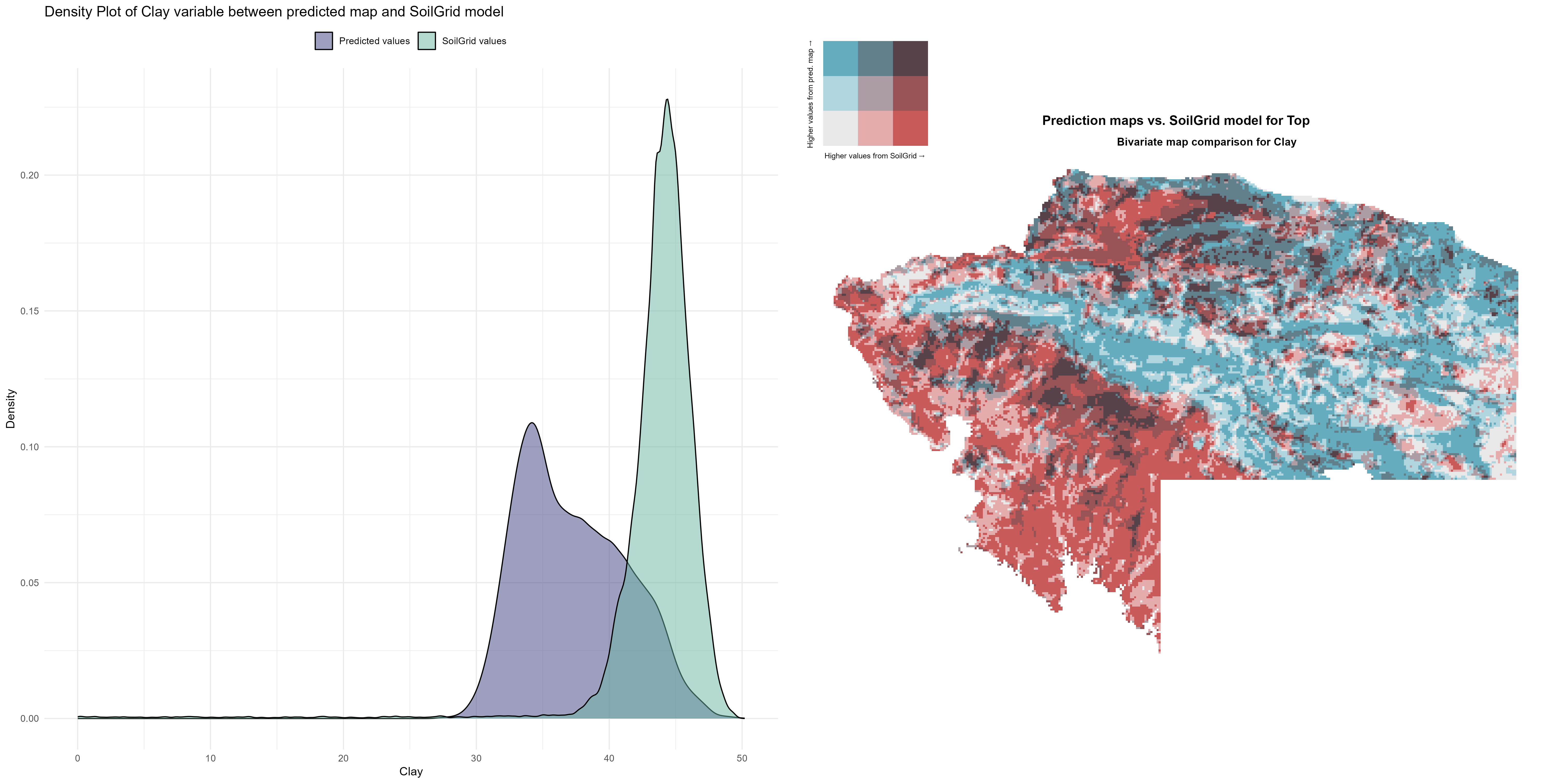
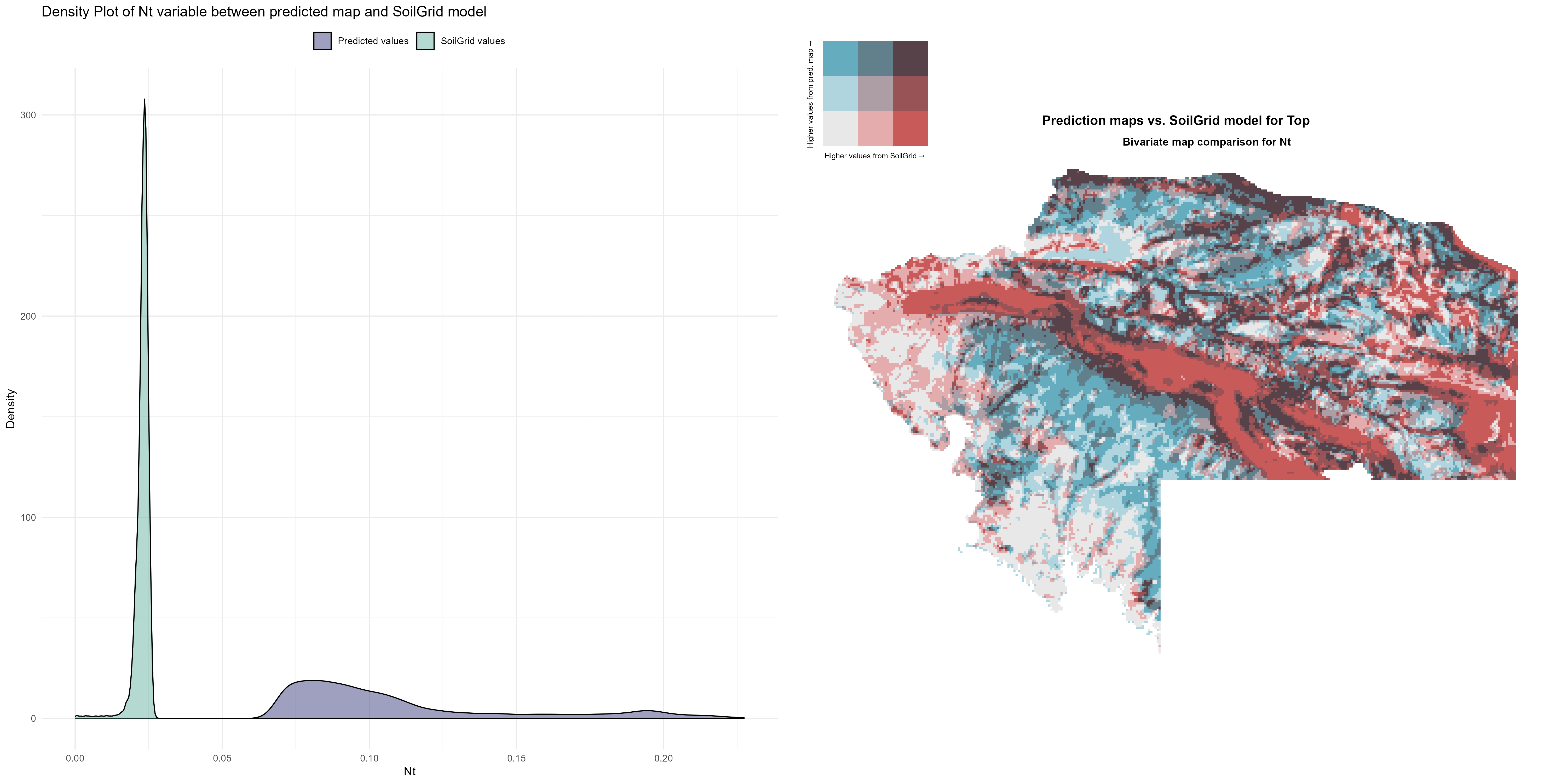
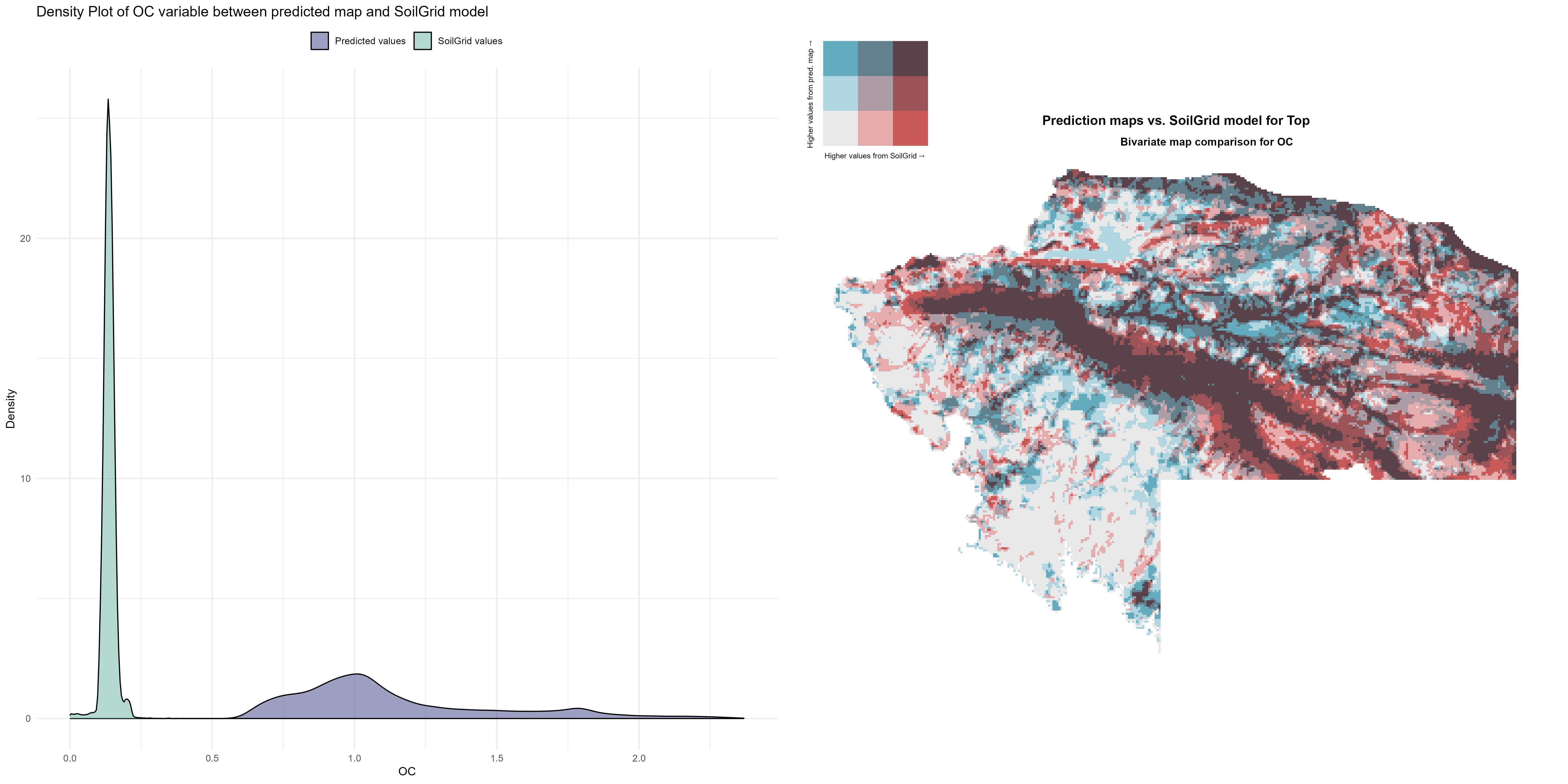
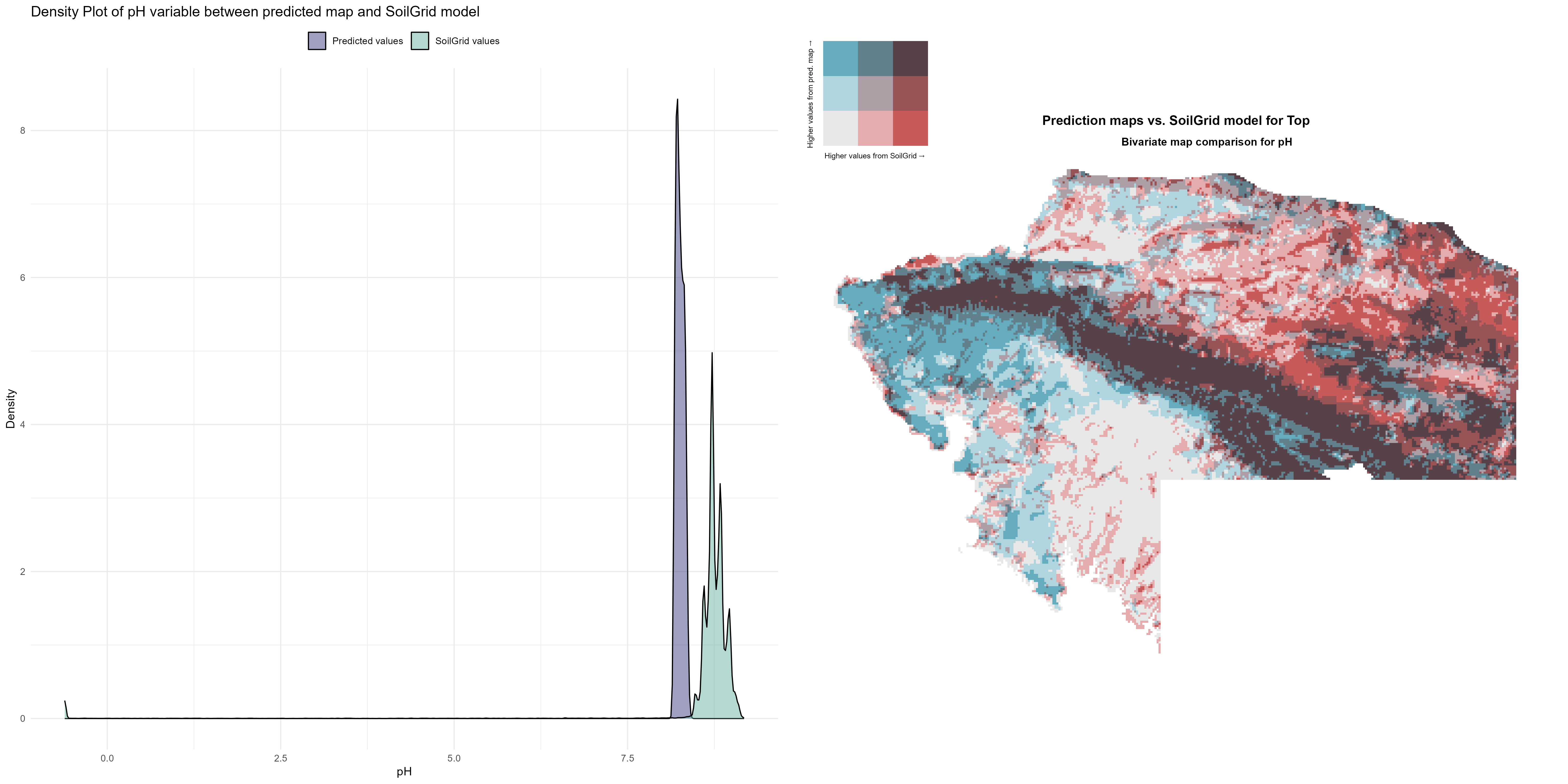
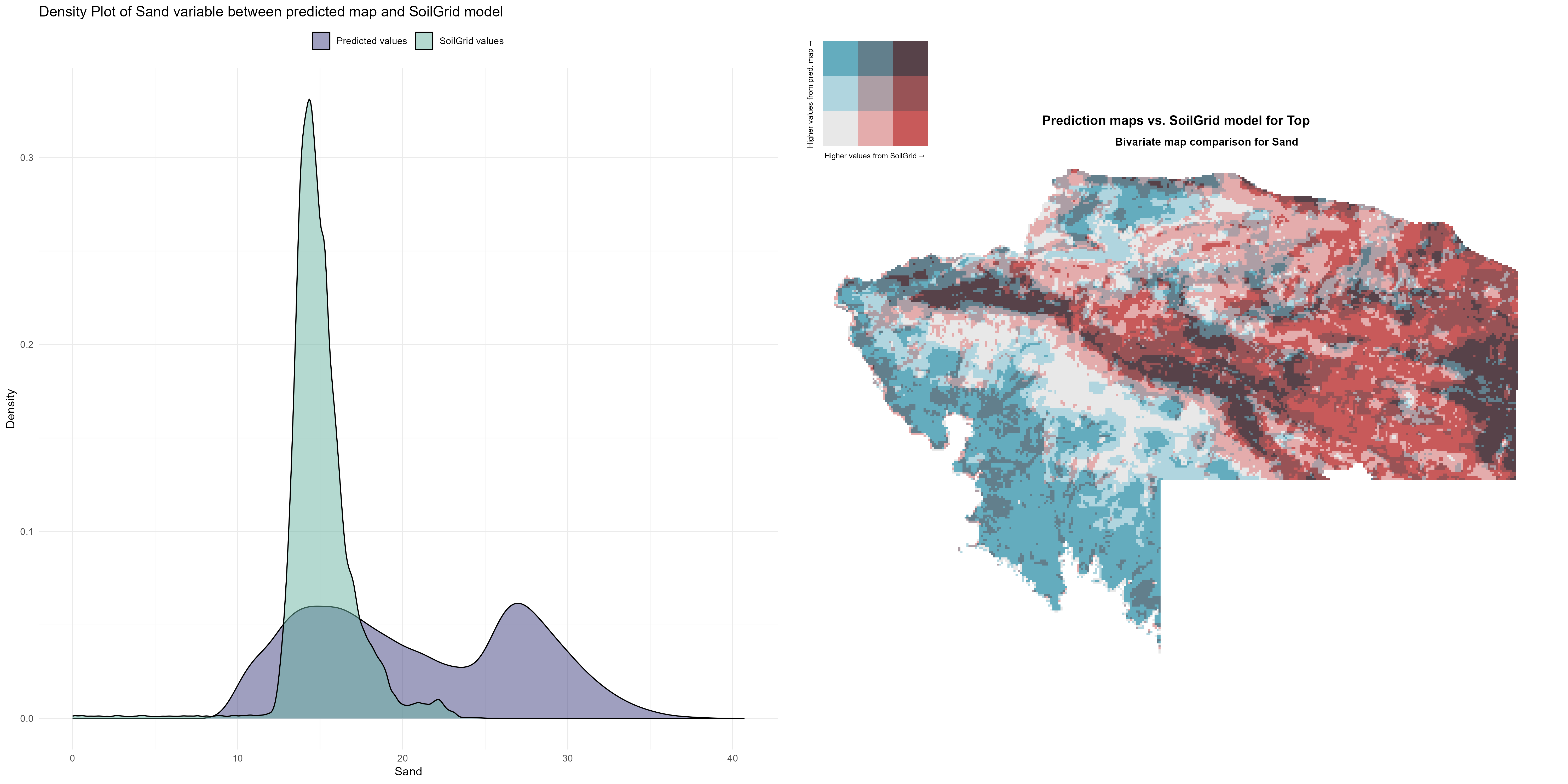
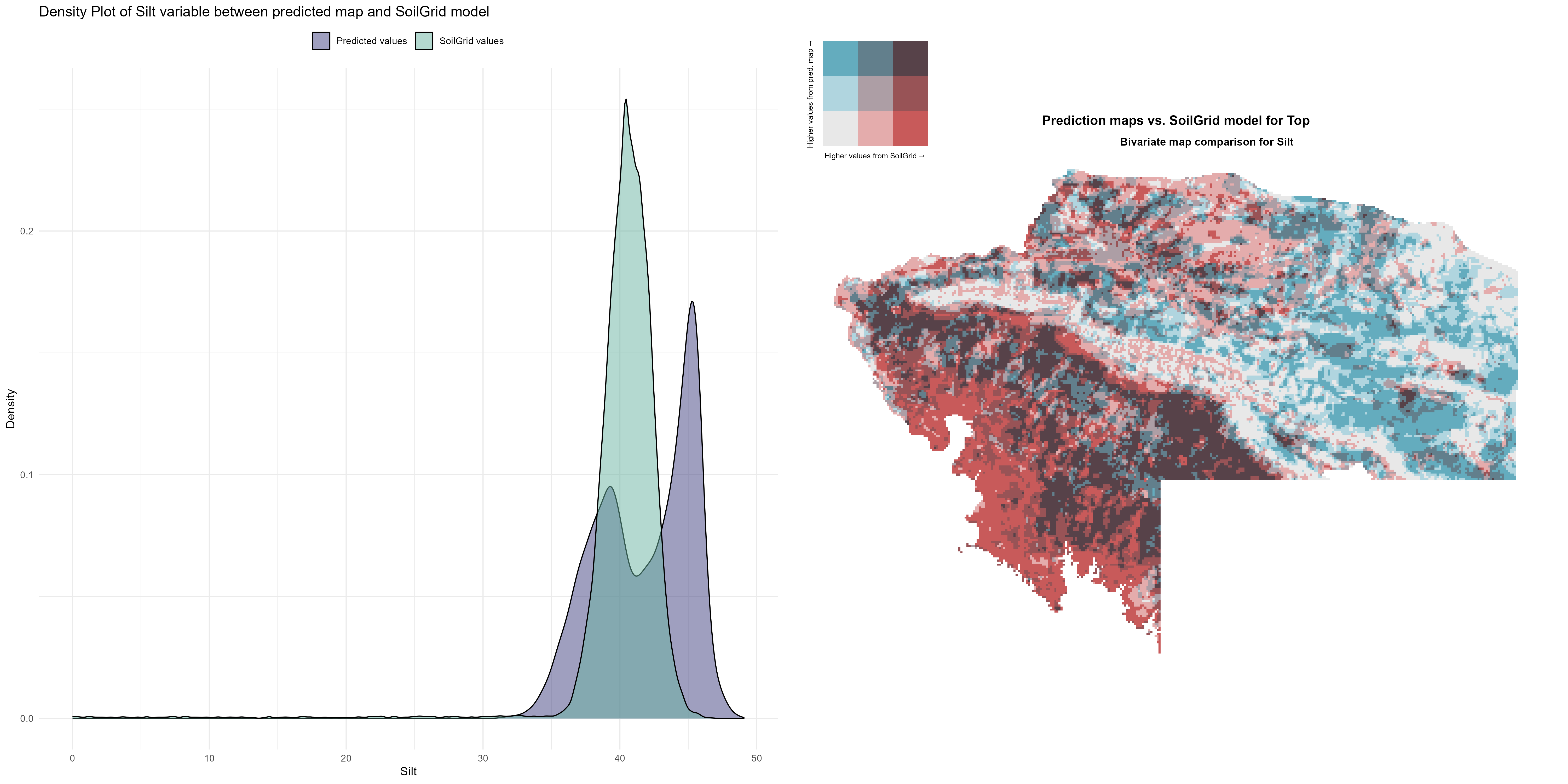
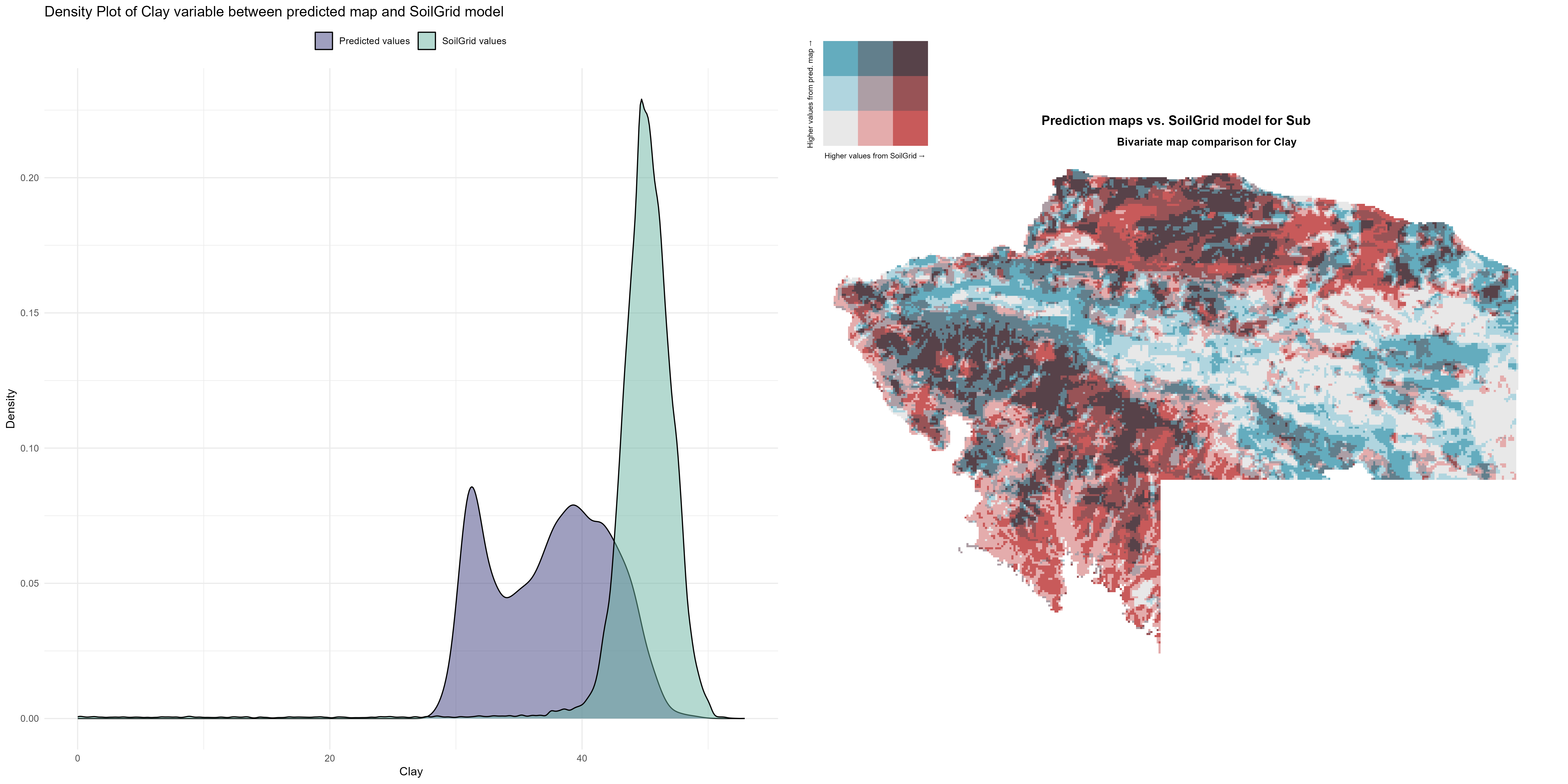
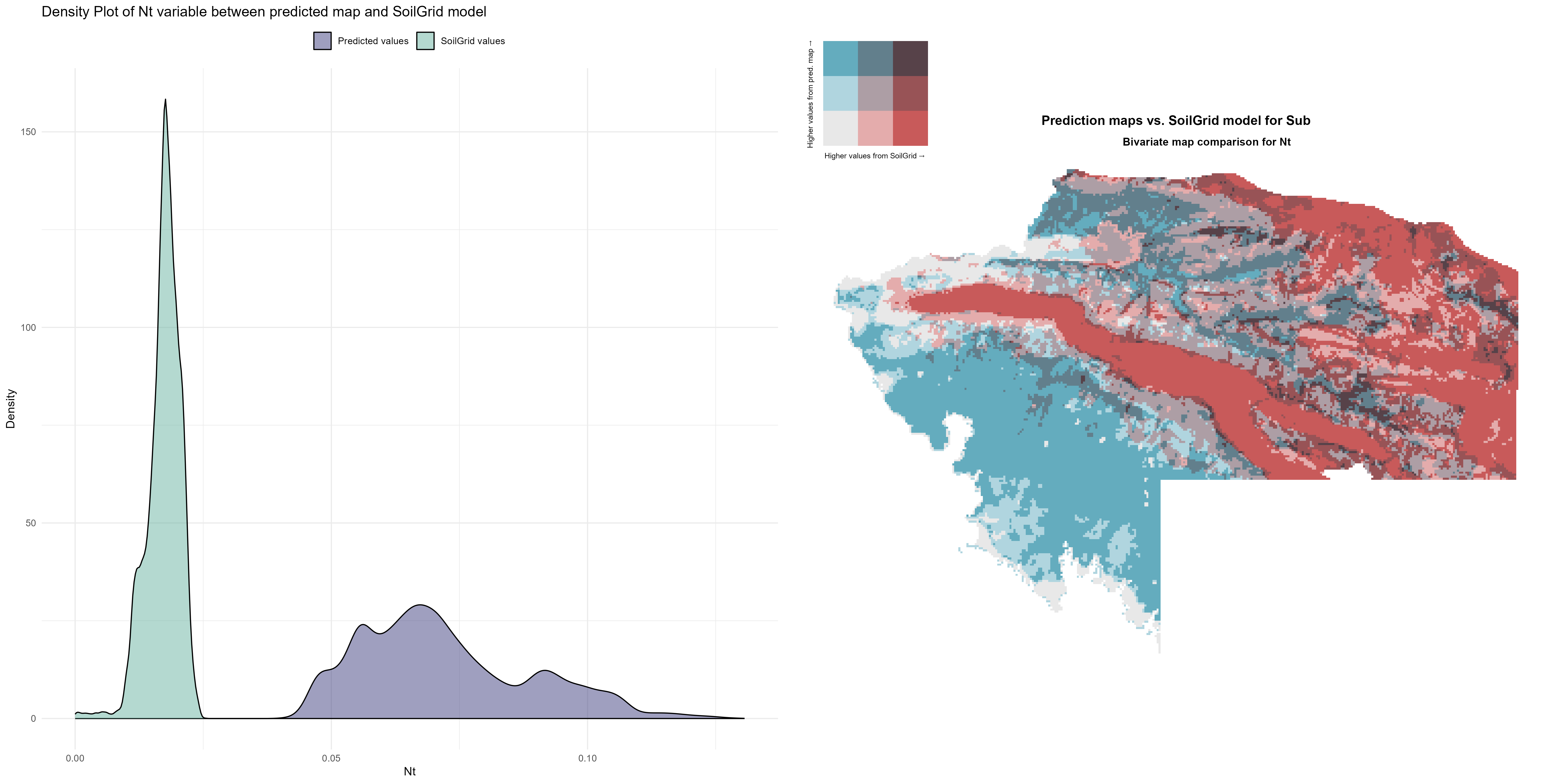

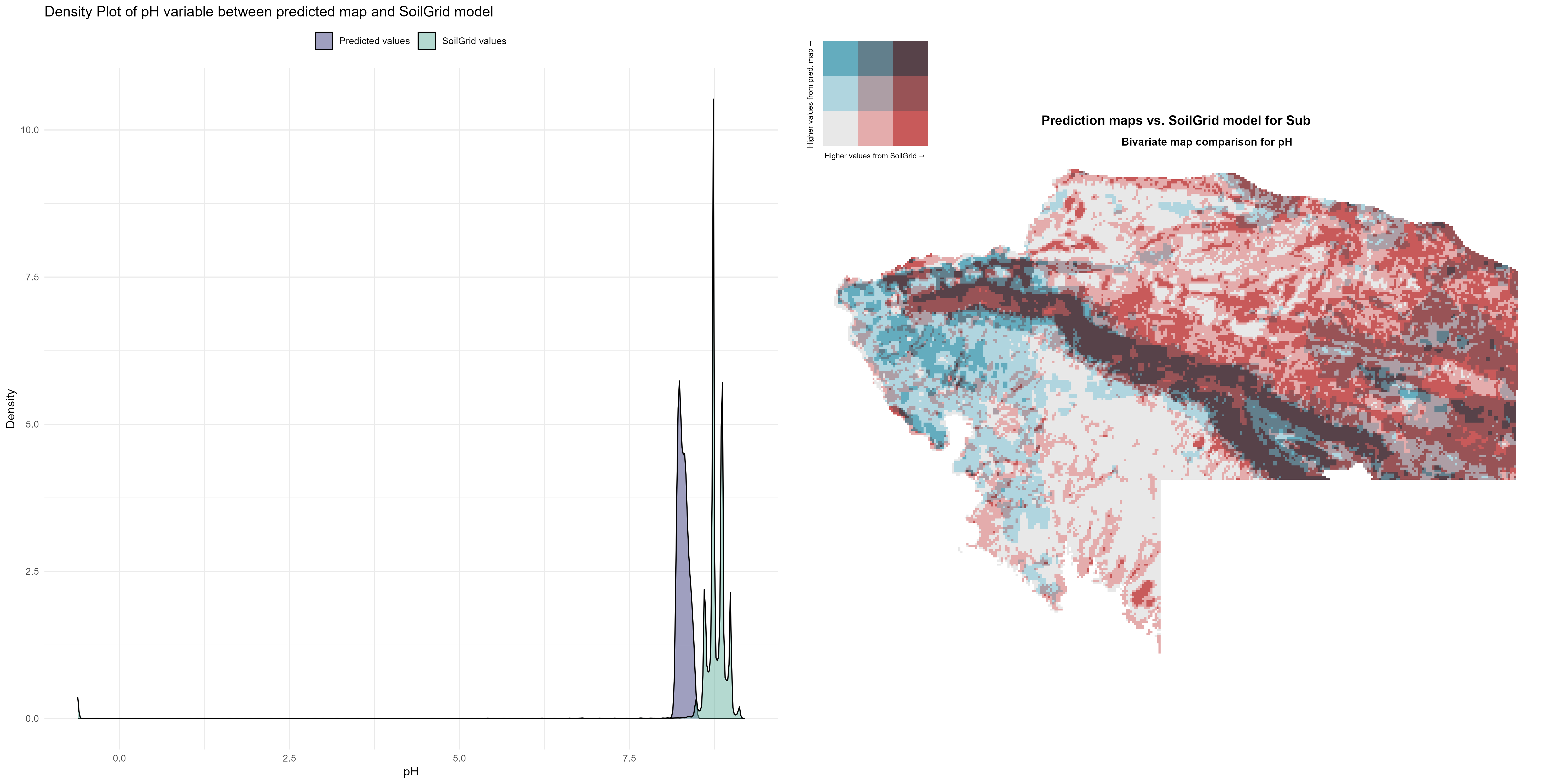


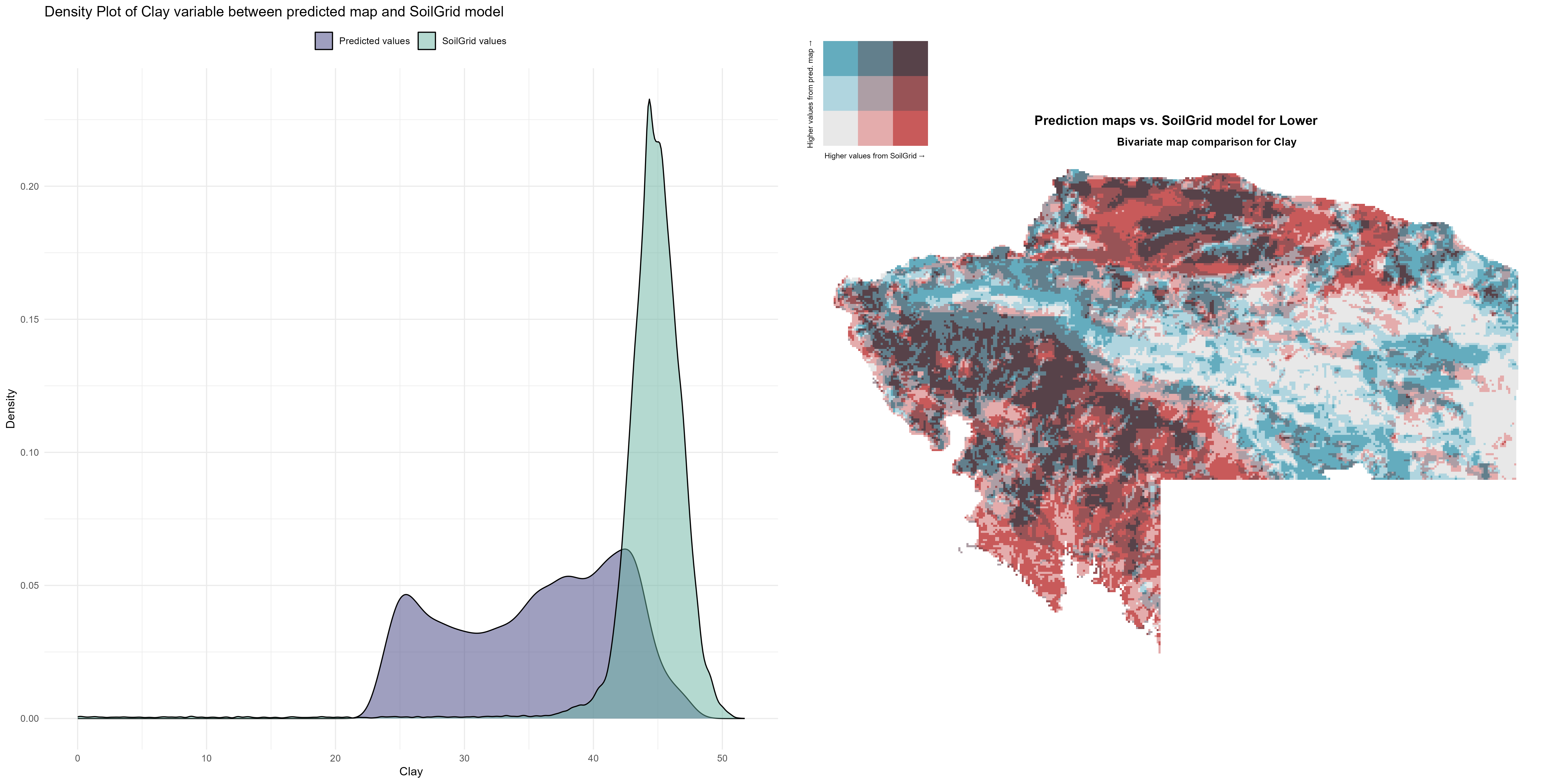
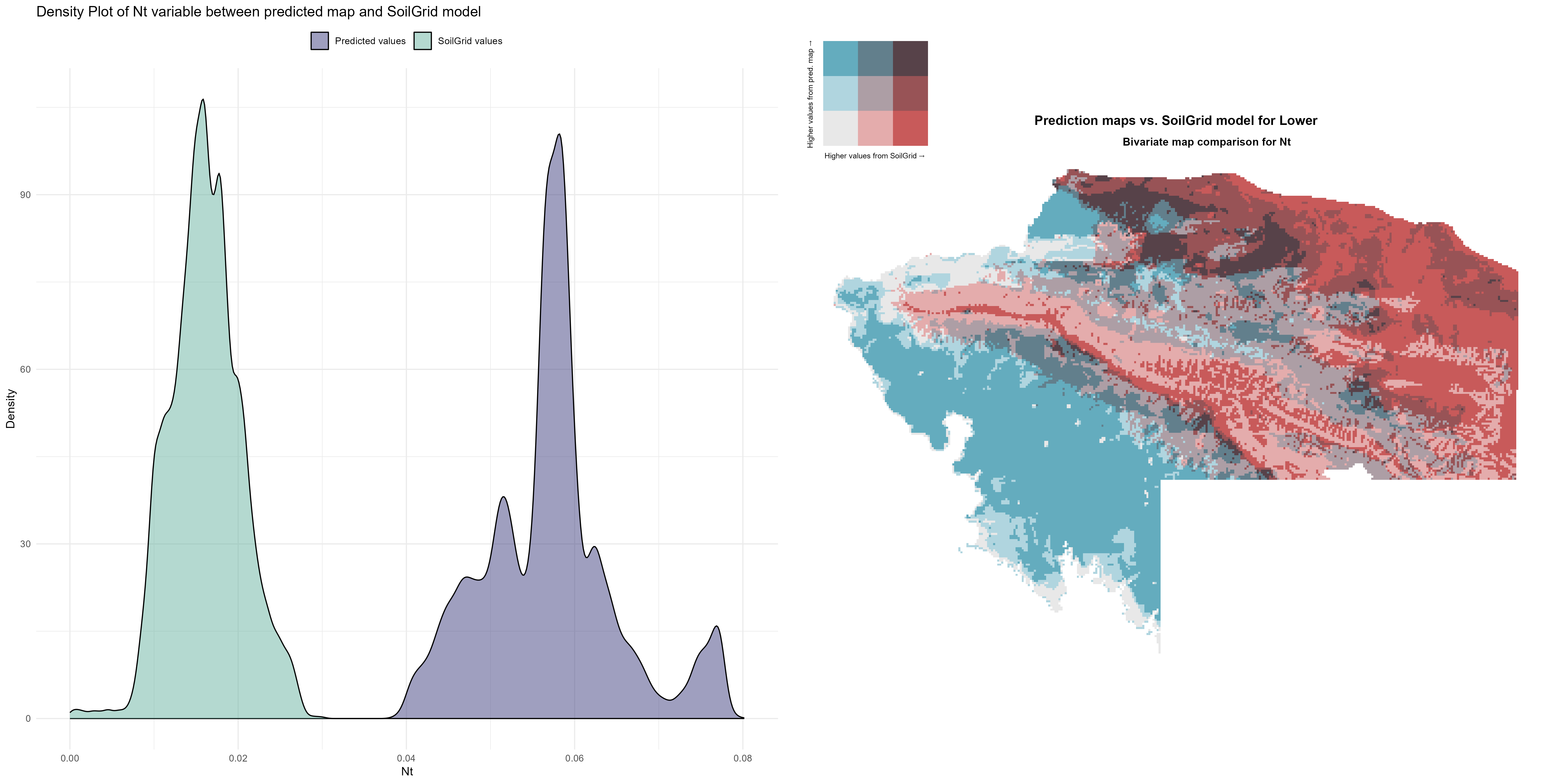
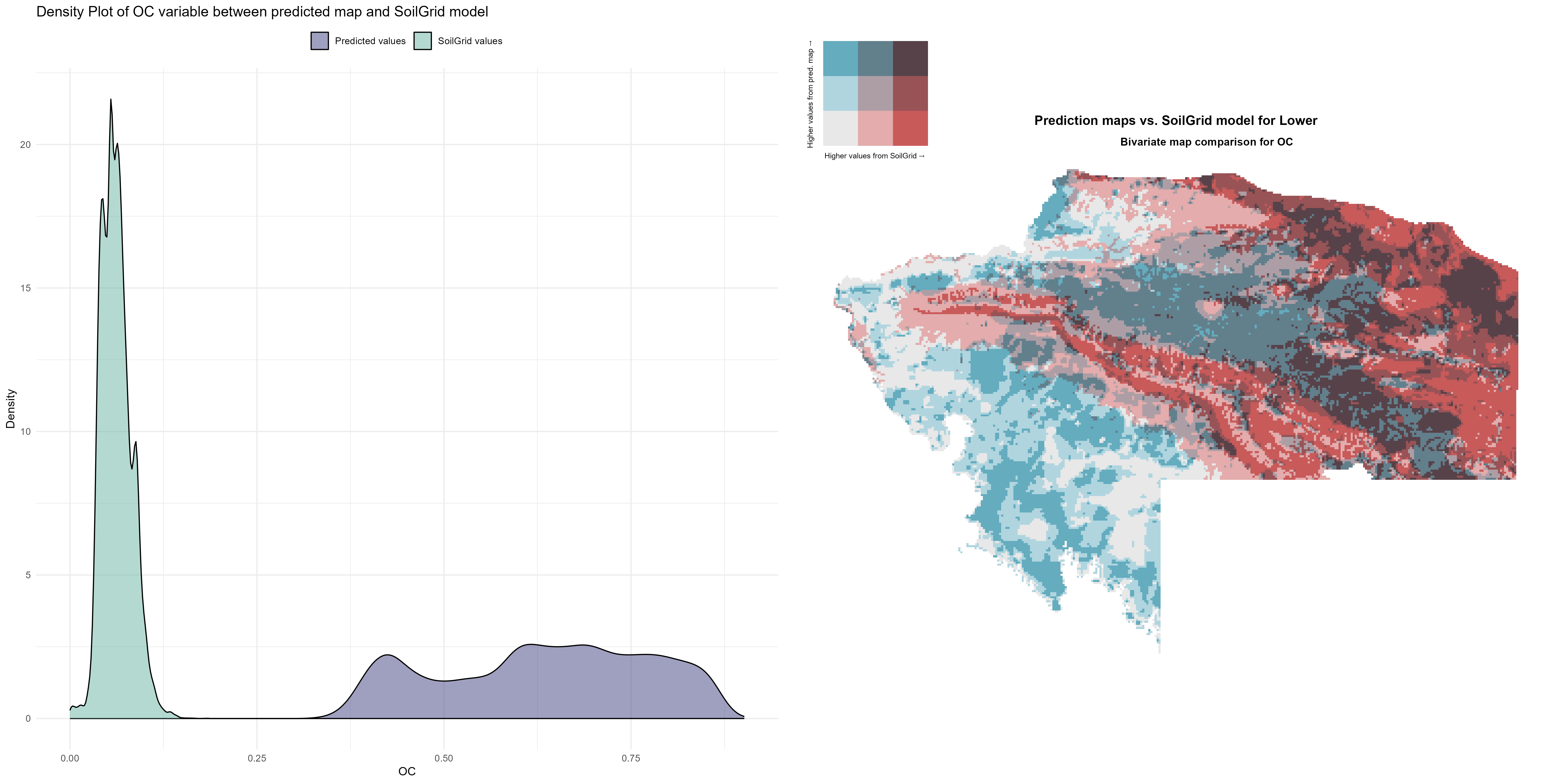
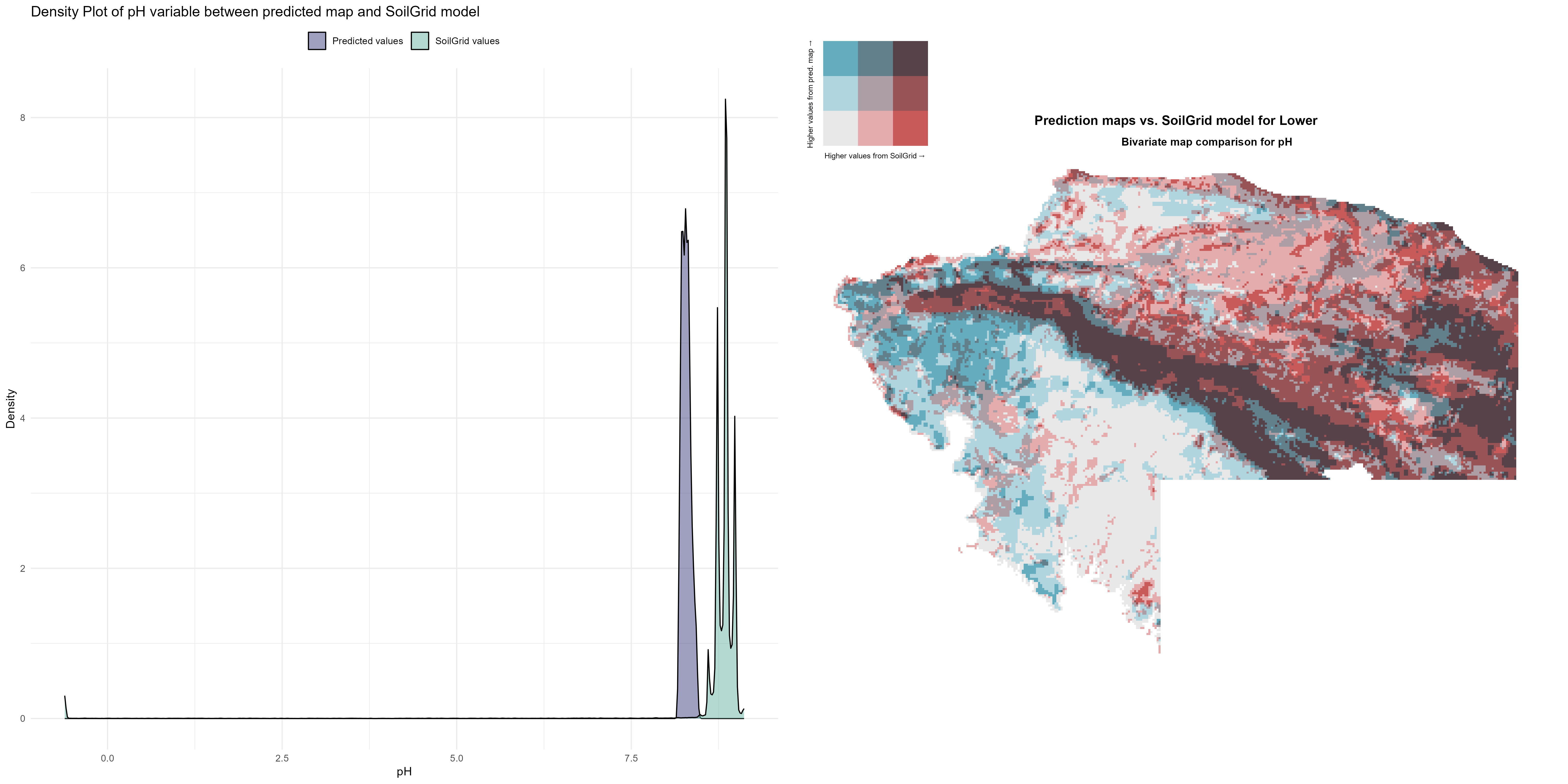


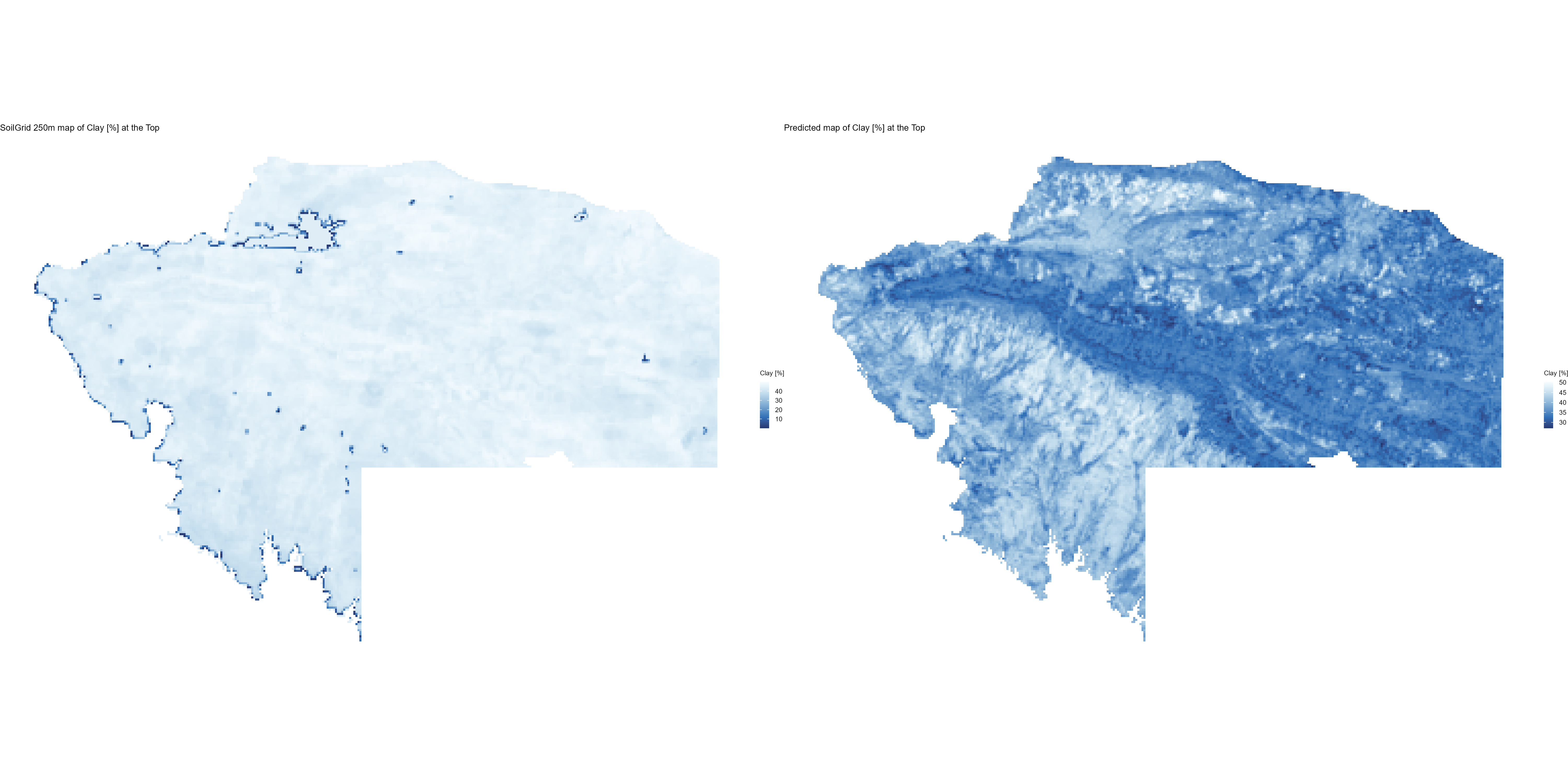
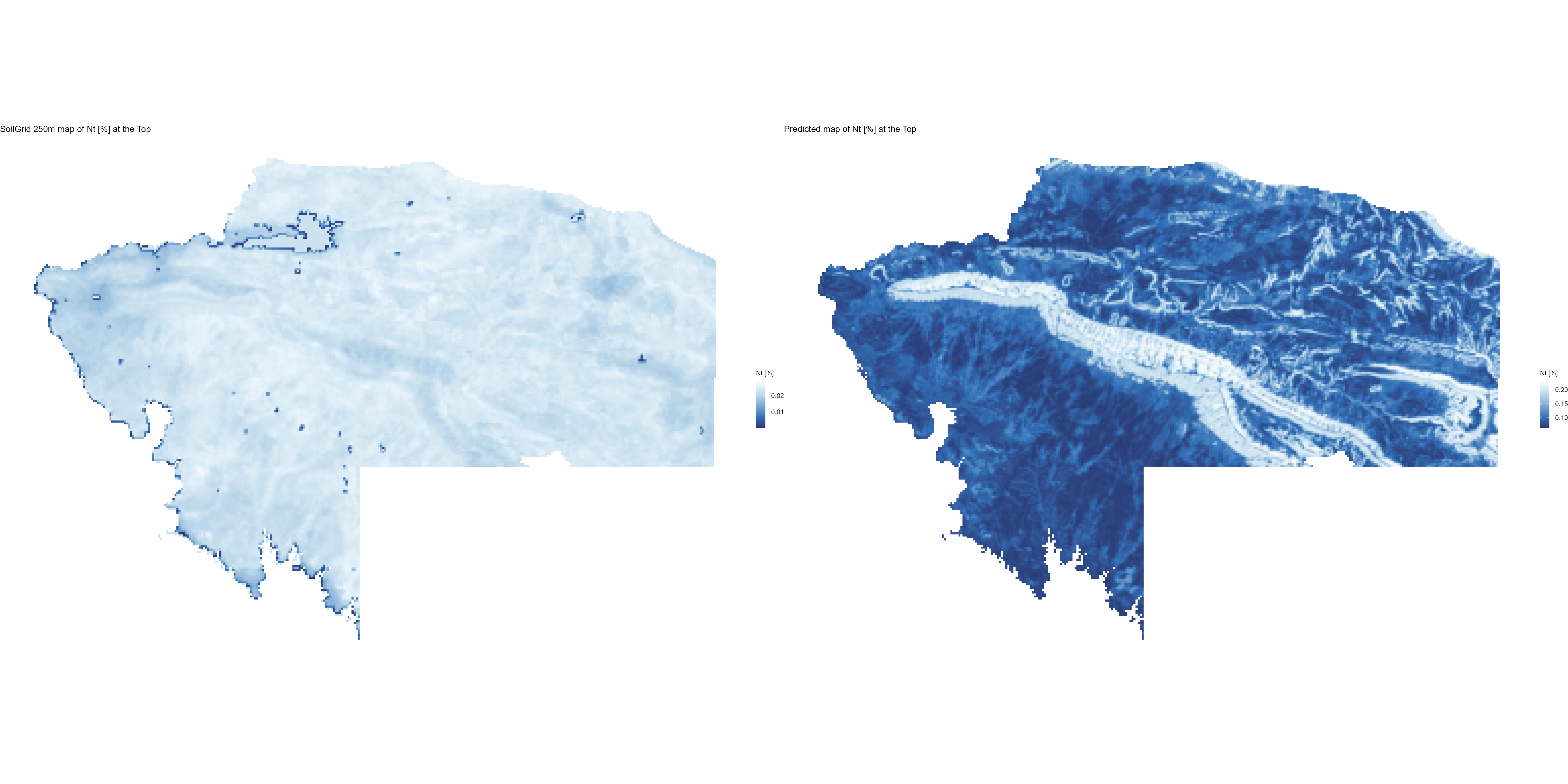
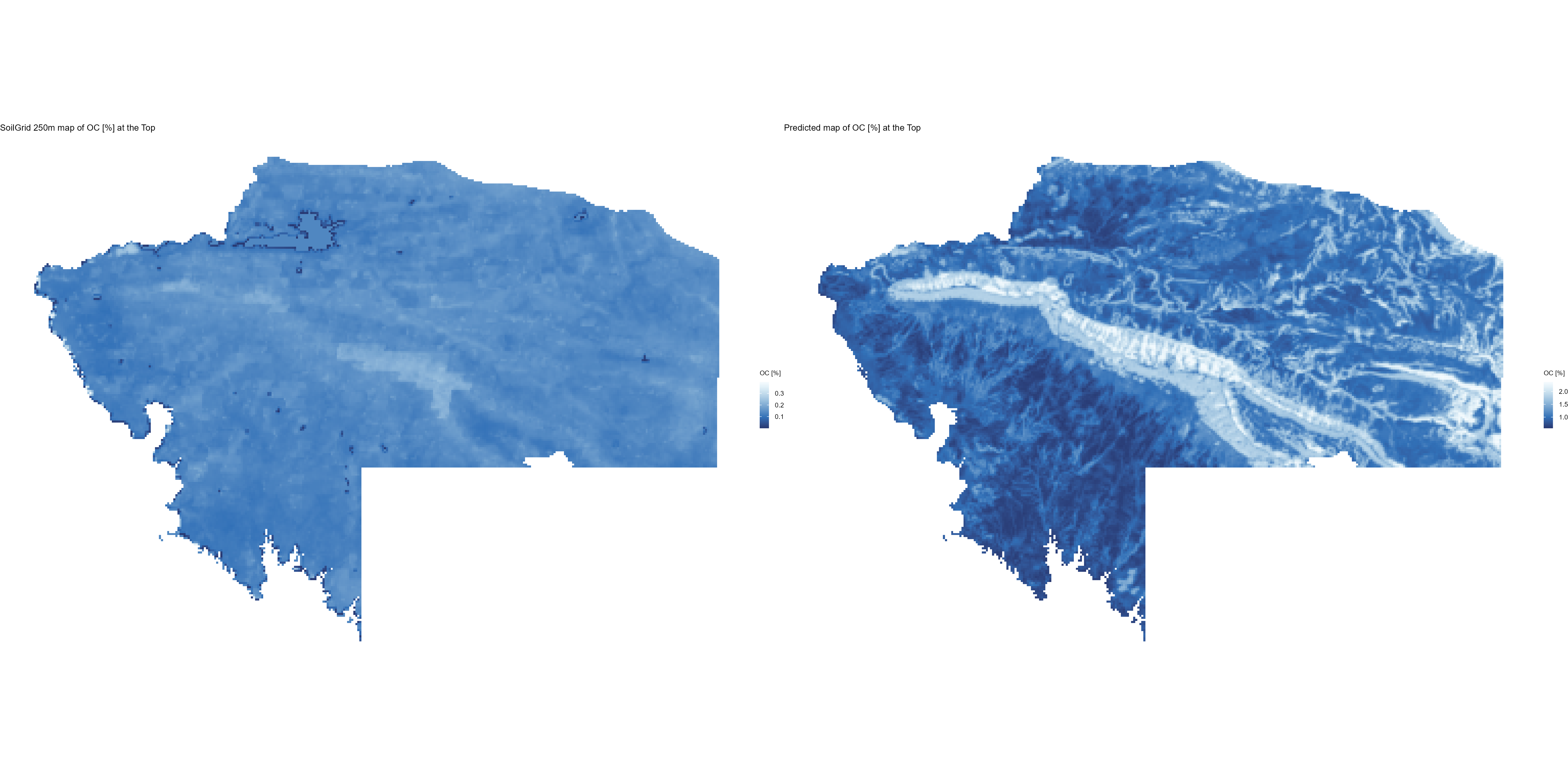
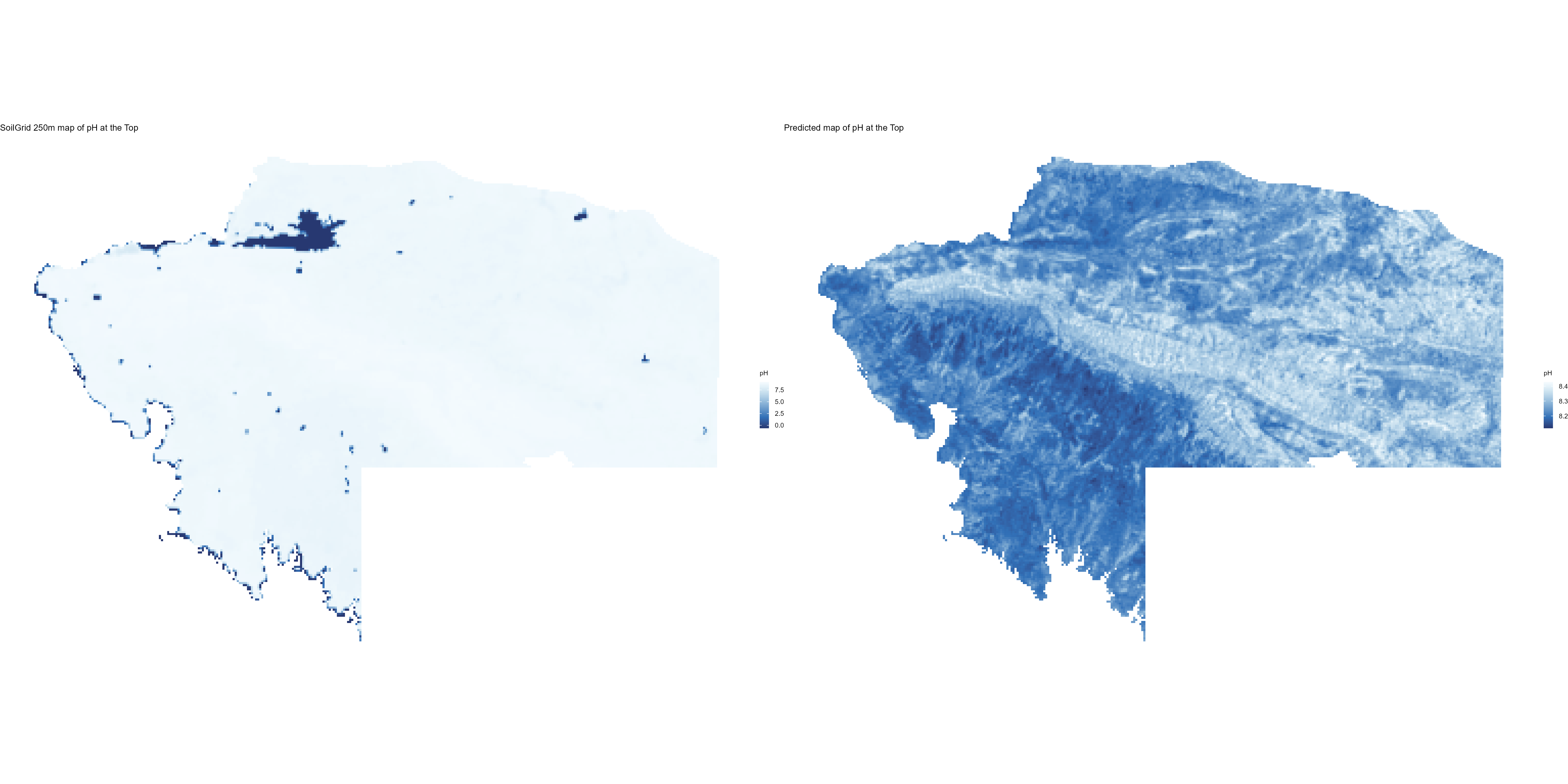
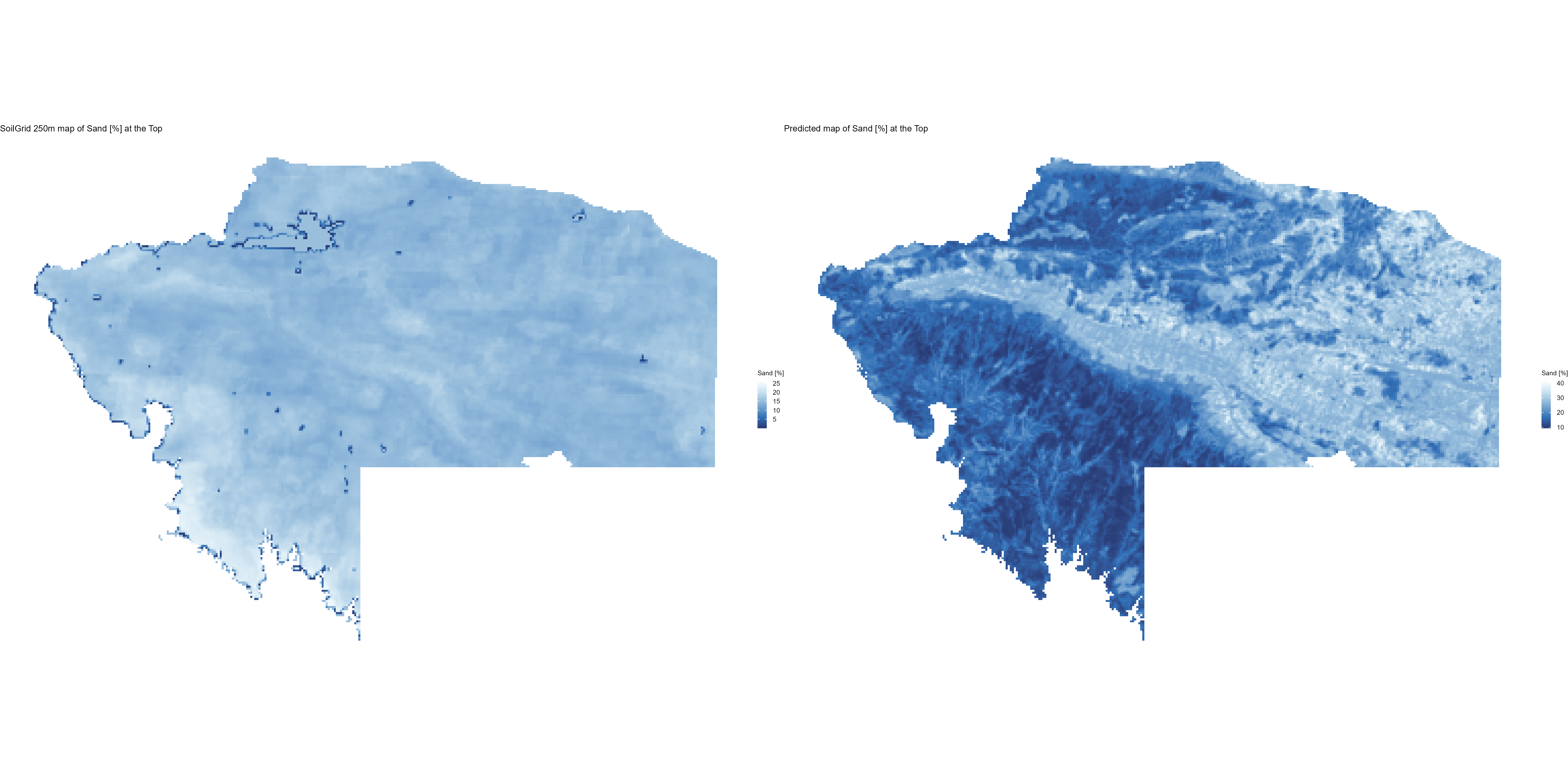
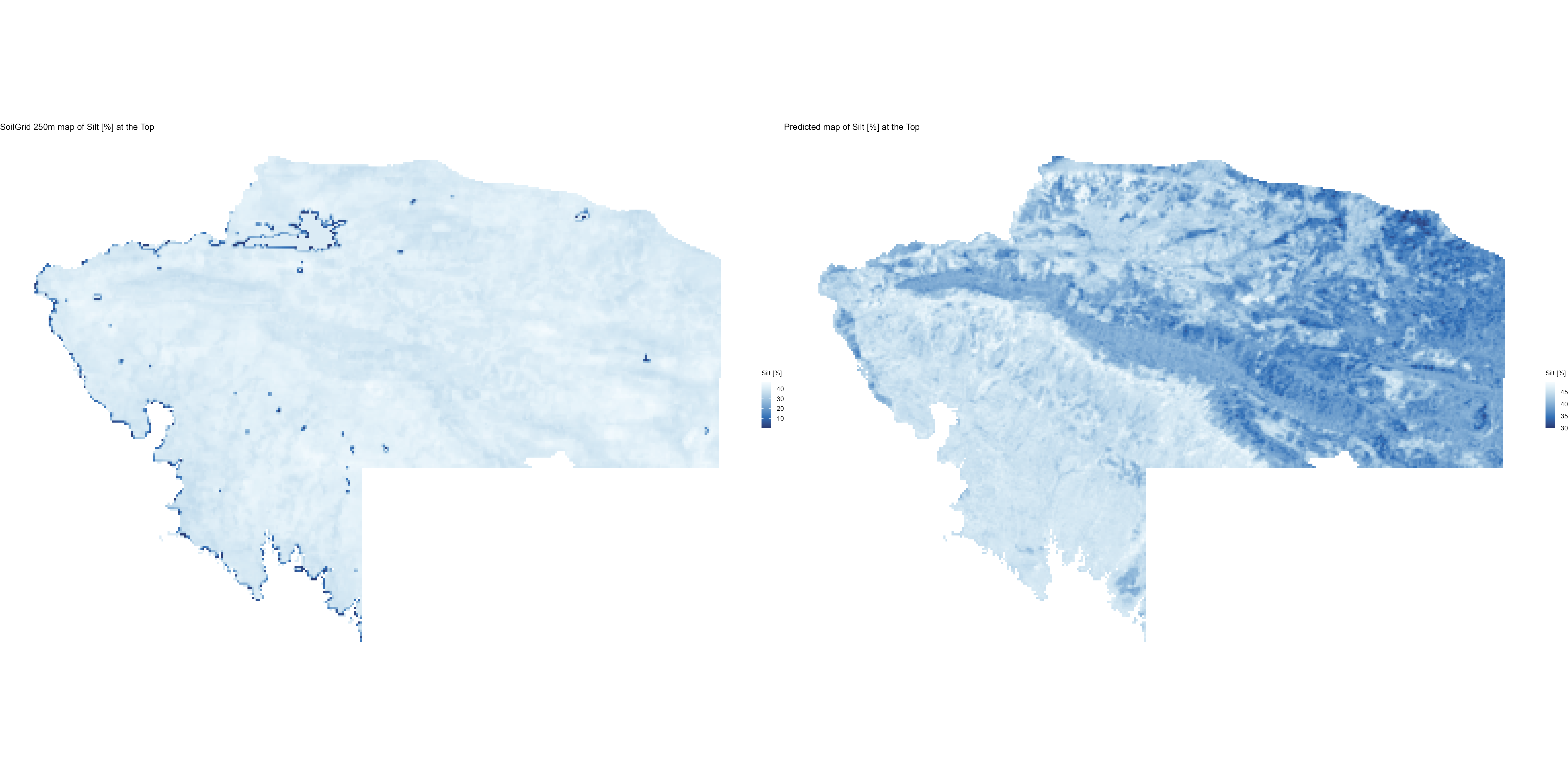
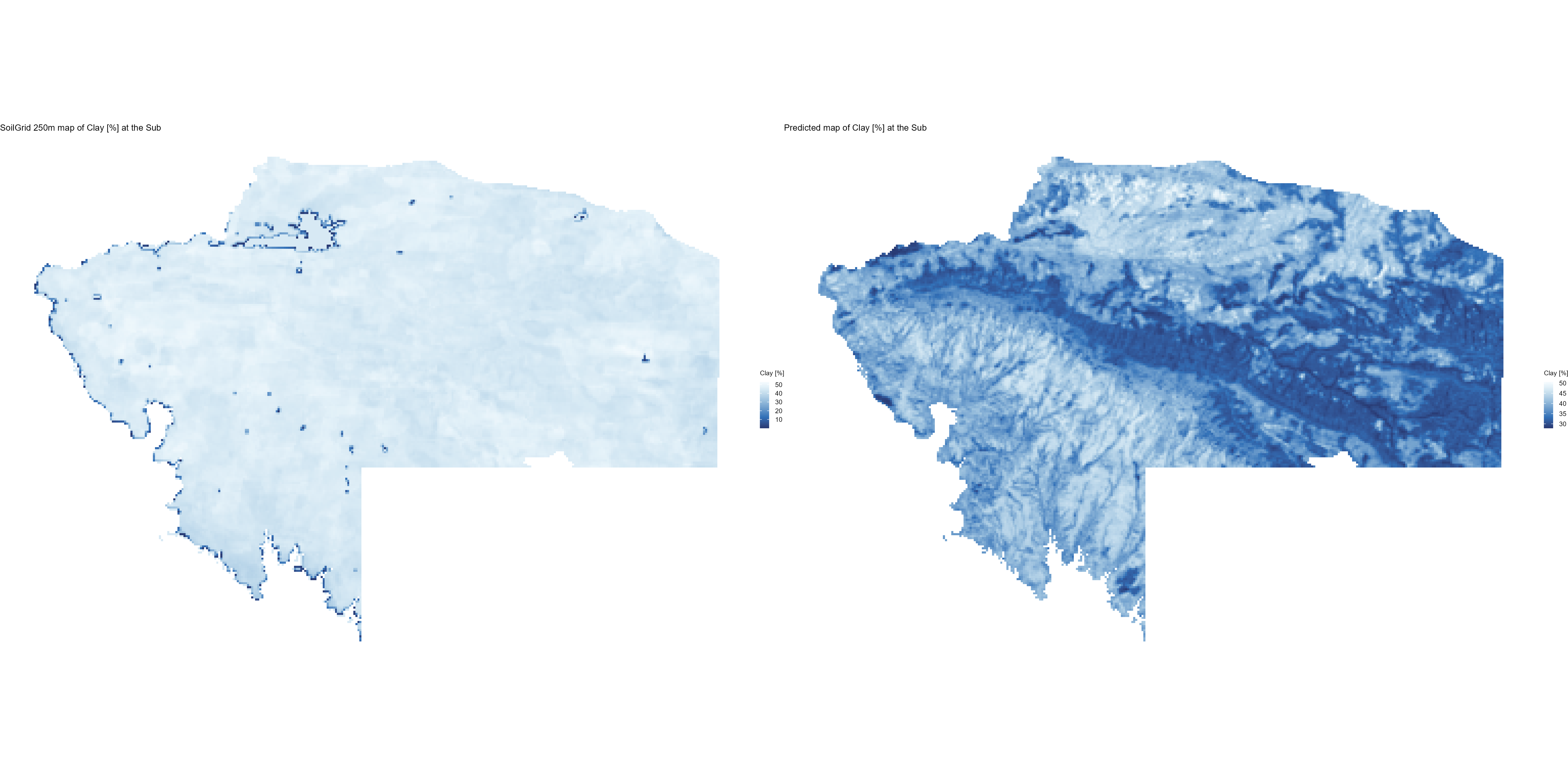
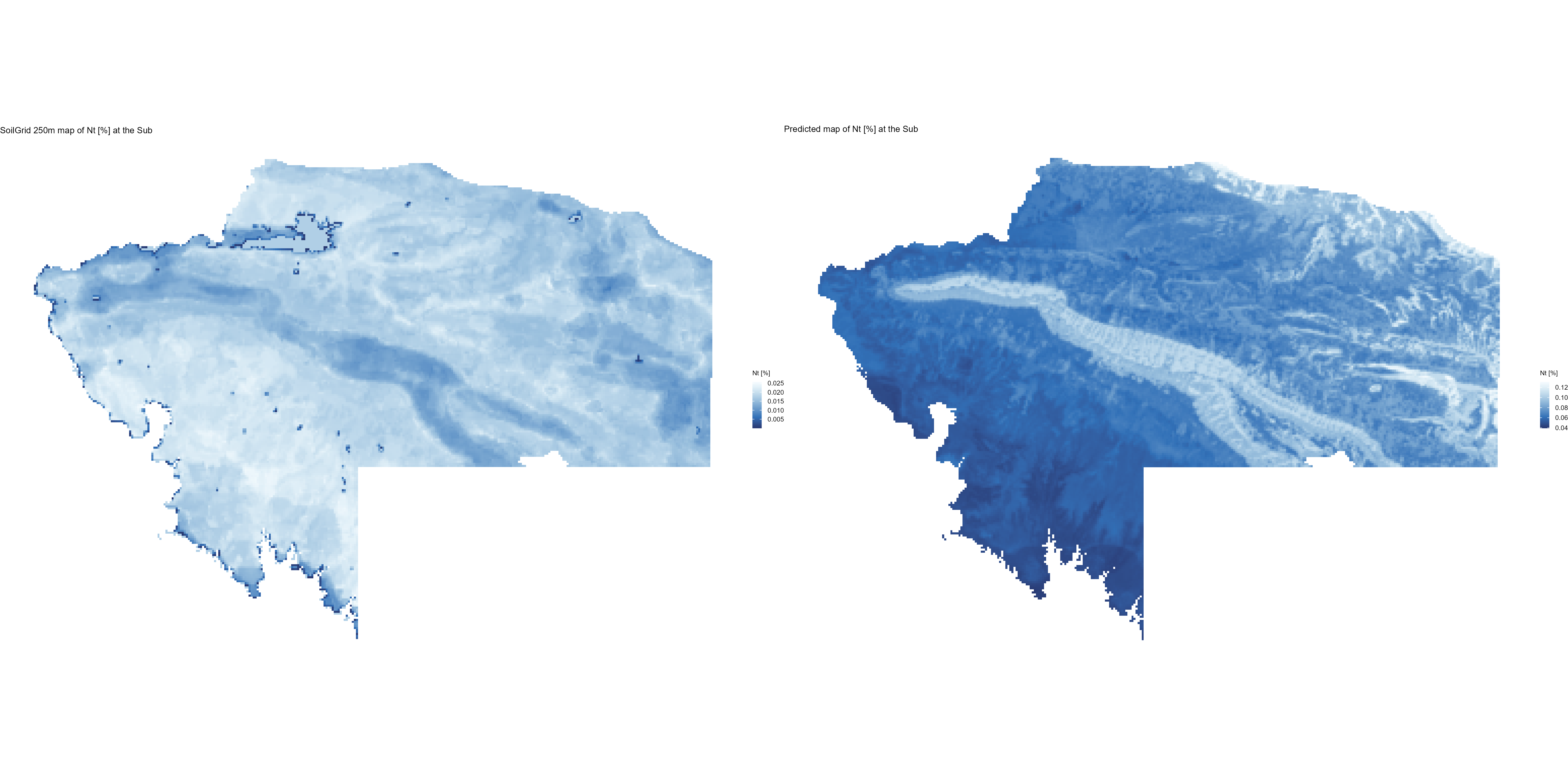
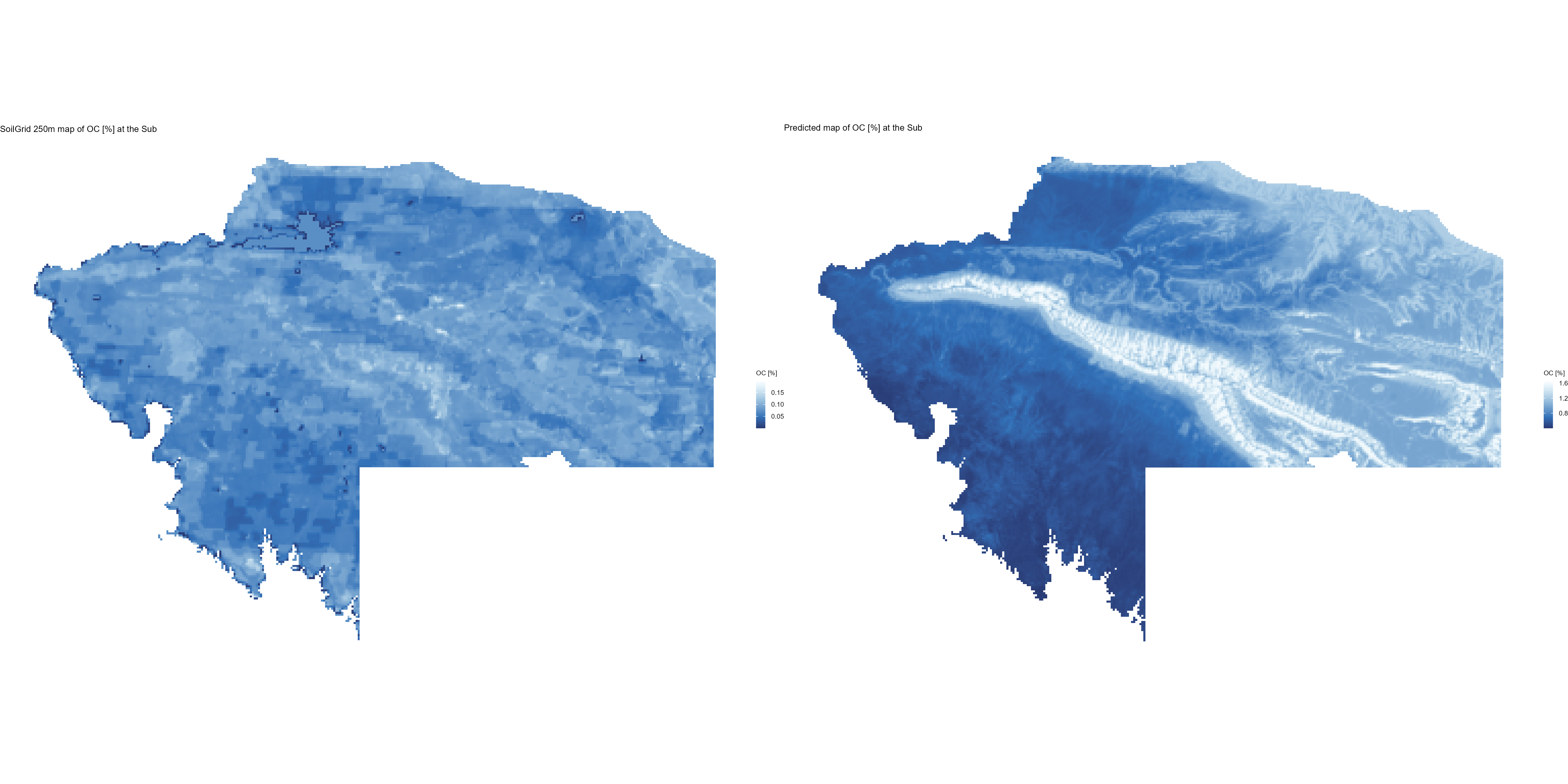
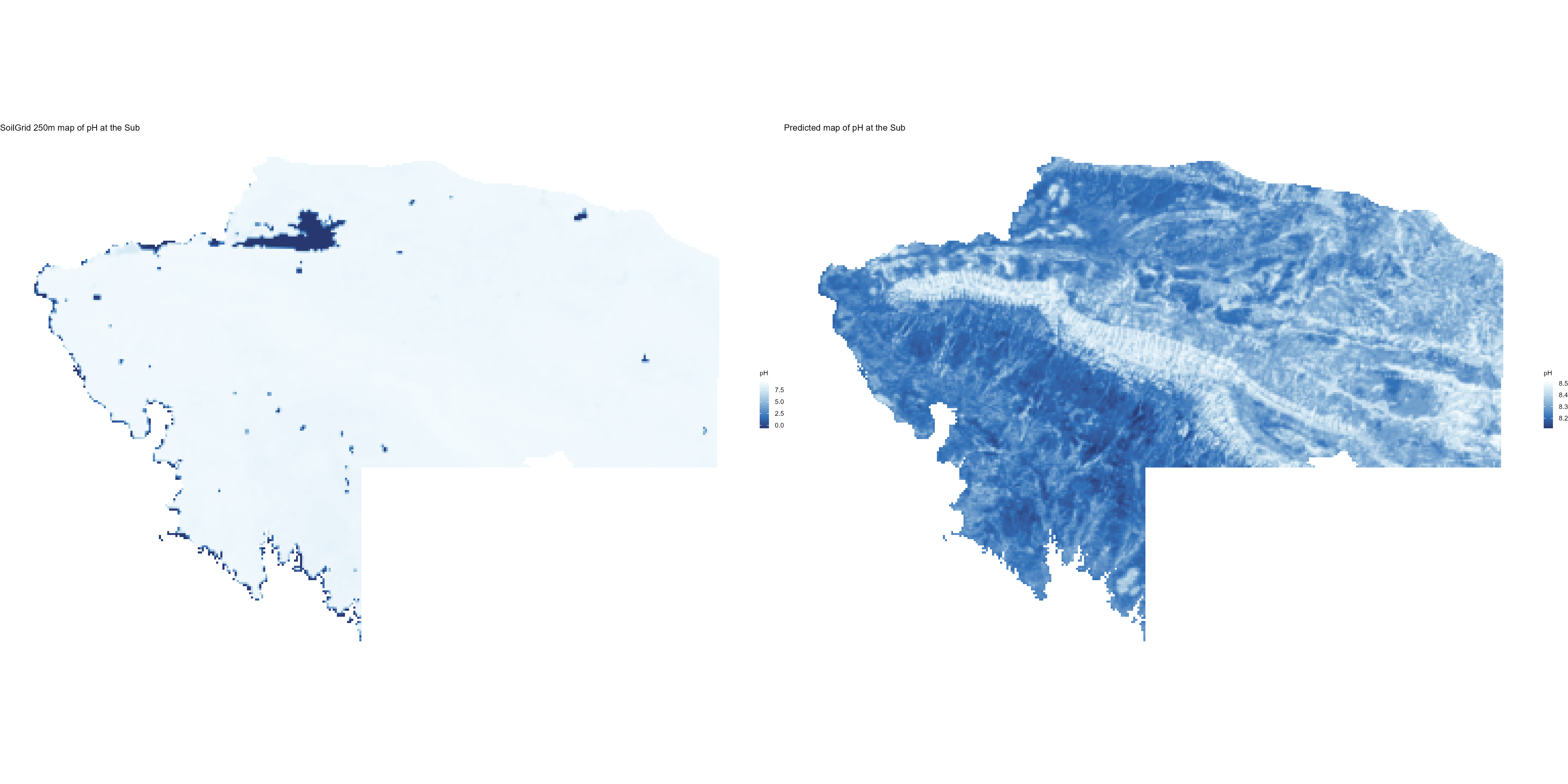
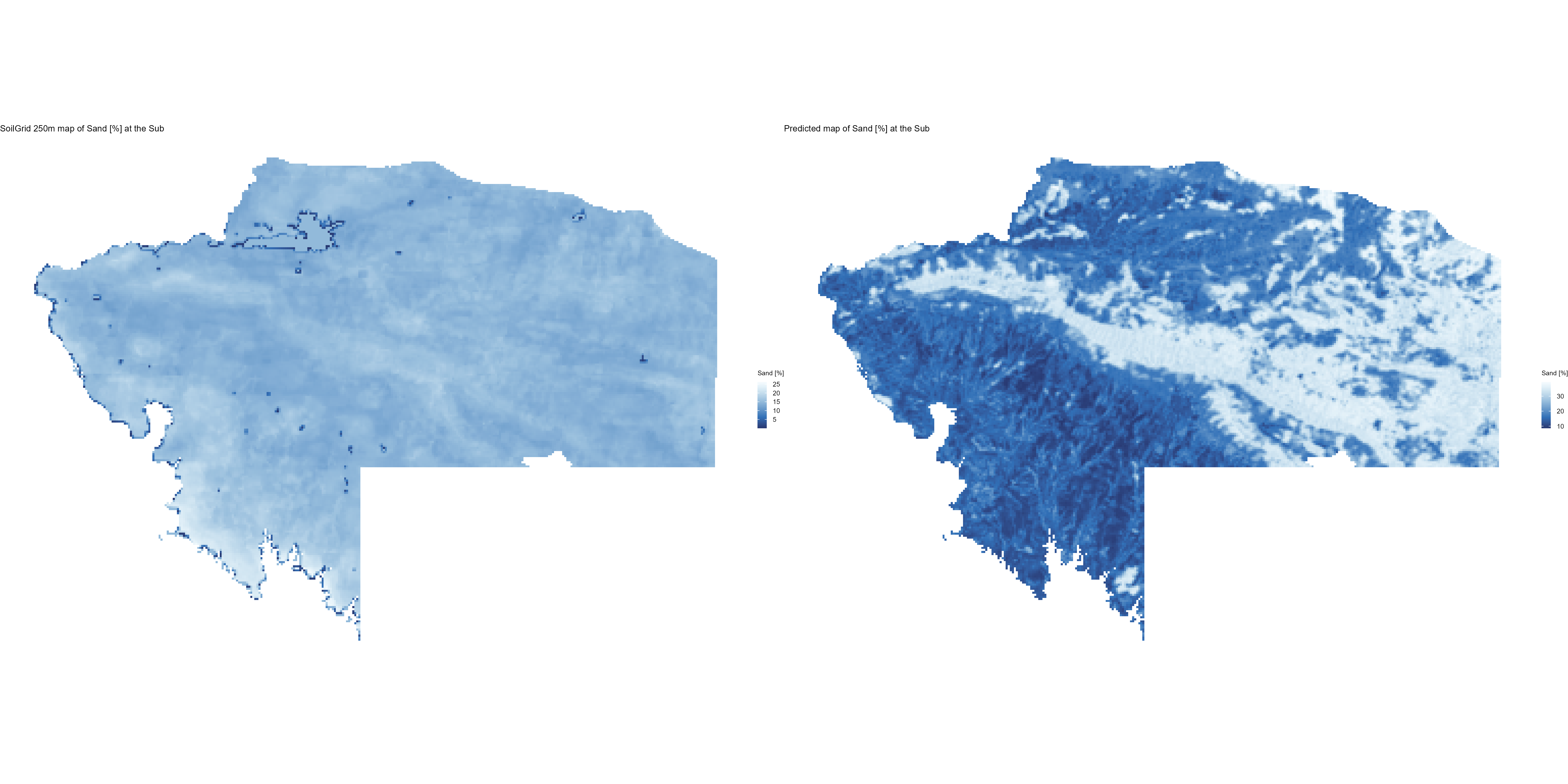


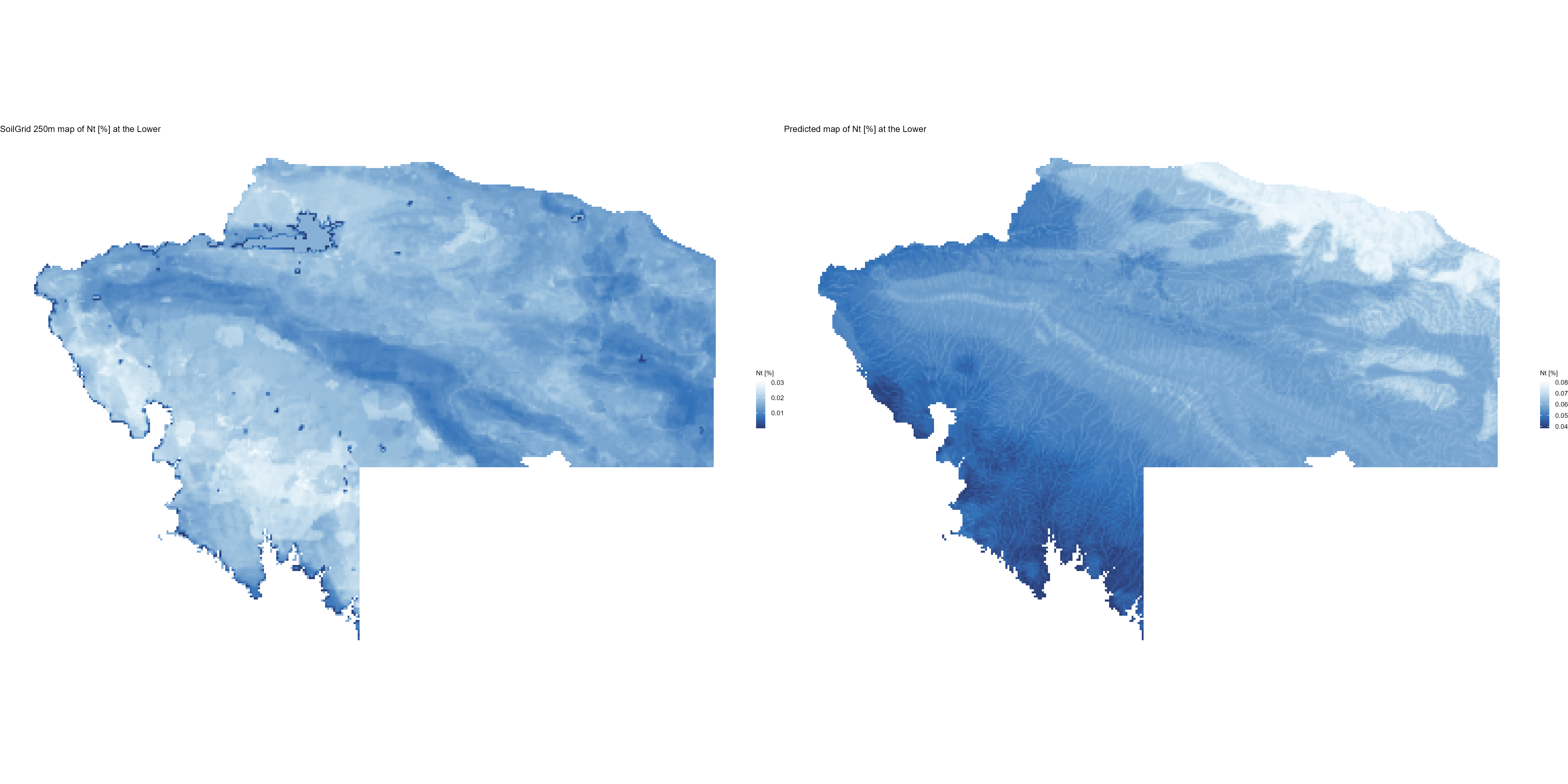
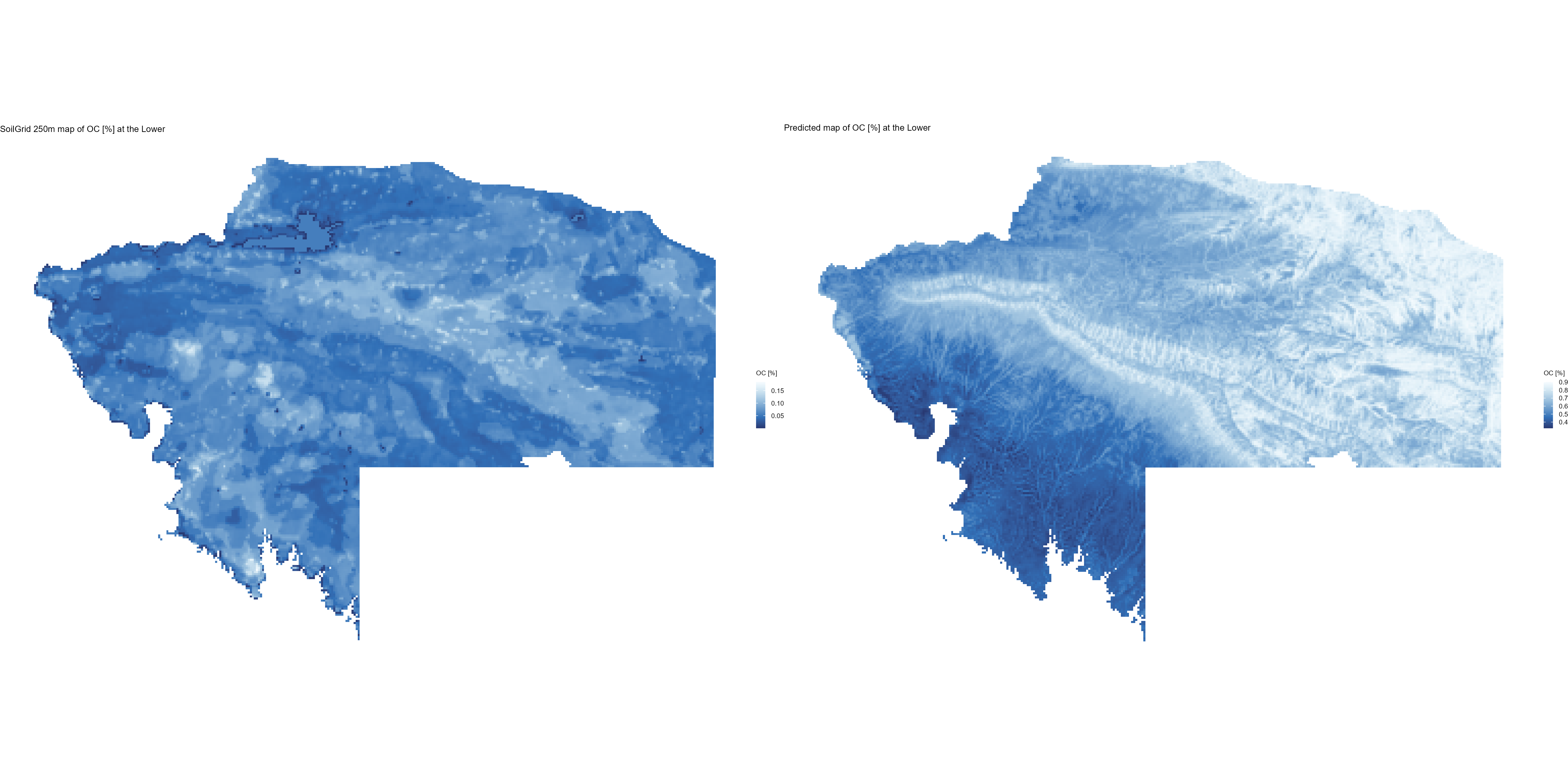
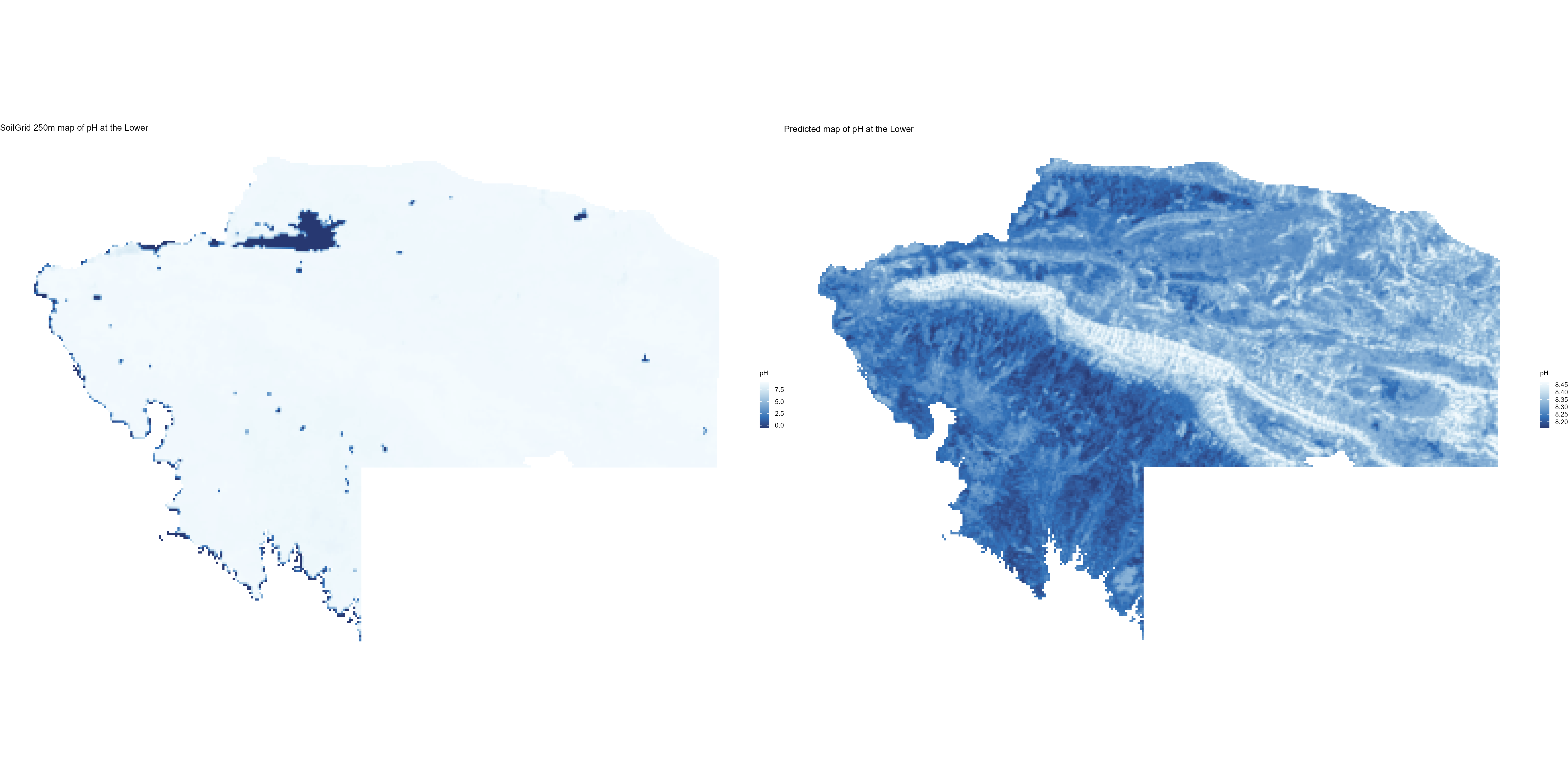
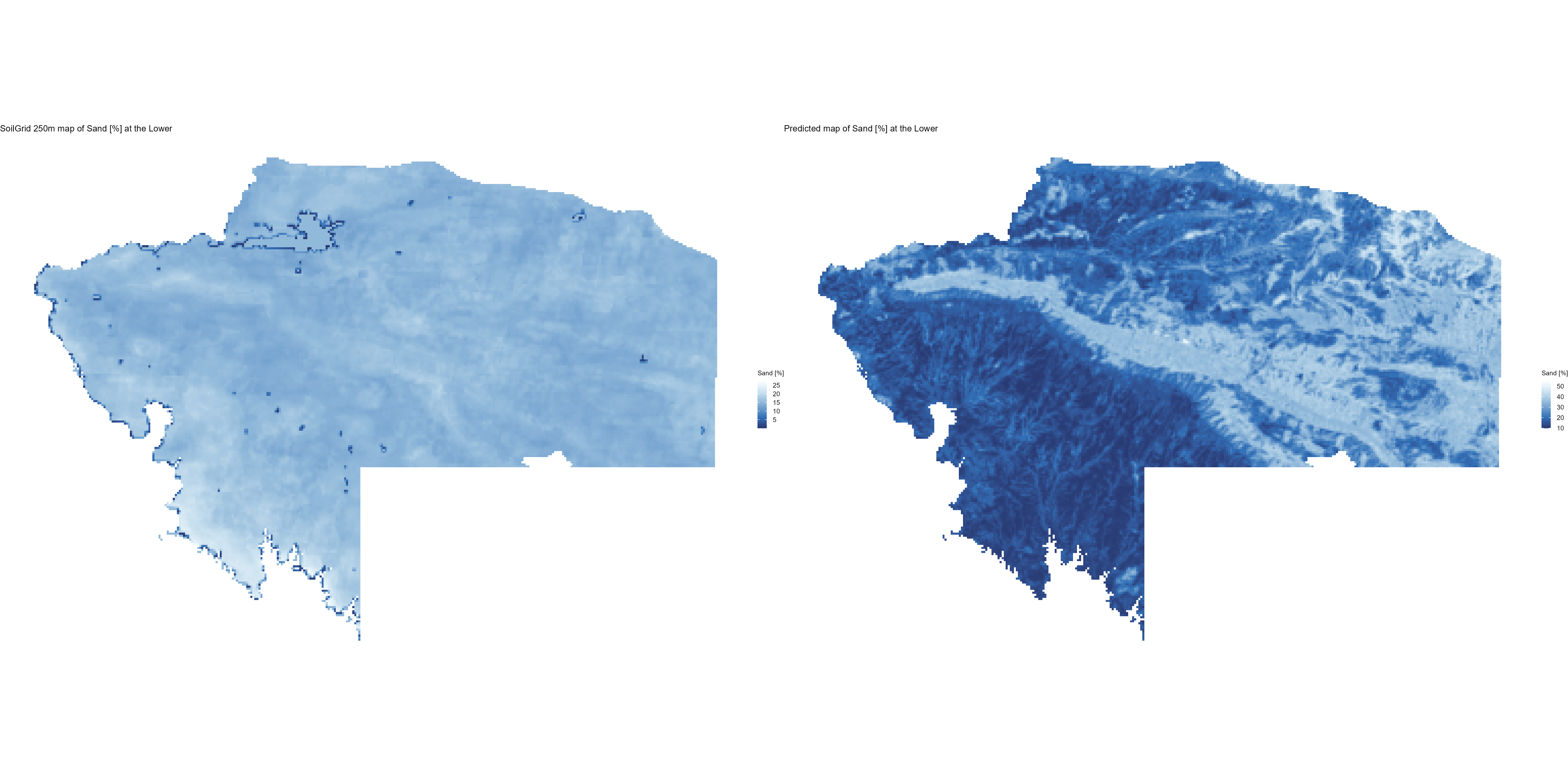
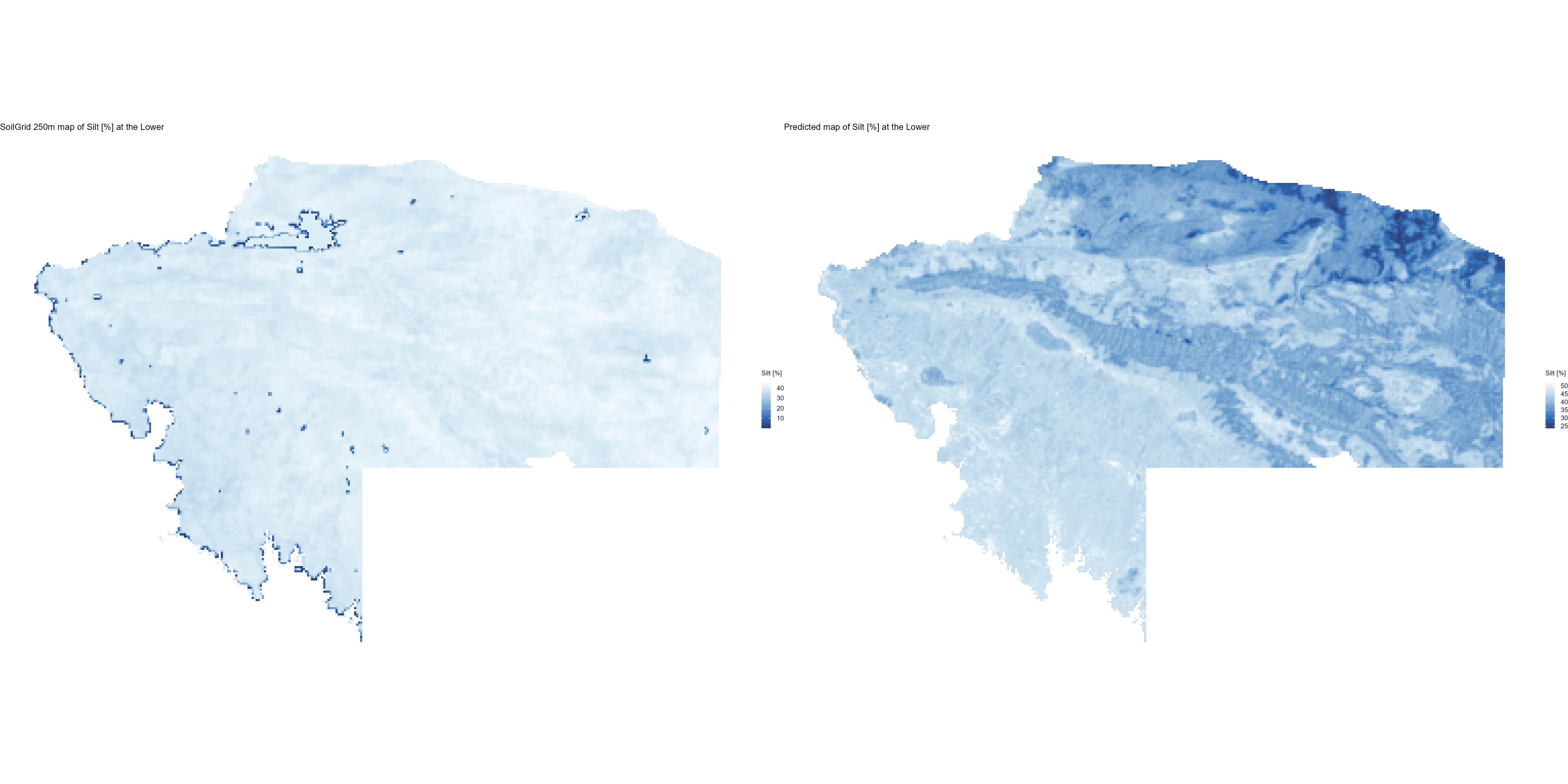
# 09.7 Plot variation of values for both maps  =================================

final.map <- List_map[[1]][,c(1:2)]
Bi_class_map <- list()

# Repeat for each variables names. The command 'bi_class' does not work with columns number.

for (depth in new_increments) {
  bi_class_df <- bi_class(List_map[[depth]], x = Clay, y = SoilGrid.Clay, style = "quantile", dim = 3)
  Bi_class_map[[depth]] <- cbind(Bi_class_map[[depth]], bi_class_df[,length(bi_class_df)])
}


for (depth in new_increments) {
  Bi_class_map[[depth]] <- as.data.frame(Bi_class_map[[depth]])
  colnames(Bi_class_map[[depth]]) <- colnames(List_map[[1]][9:14])
 for (var in colnames(List_map[[1]][9:14])) {
   split_result <- stringr::str_split_fixed(Bi_class_map[[depth]][[var]], "-", n = 2)
   Bi_class_map[[depth]][[paste0(var, "_1")]] <- as.numeric(split_result[,1])
   Bi_class_map[[depth]][[paste0(var, "_2")]] <- as.numeric(split_result[,2])
 }
}

df <- List_map[[1]][,c(1:2)]

for (var in colnames(List_map[[1]][9:14])) {
  df[[paste0("predicted.",var)]] <- (Bi_class_map[[1]][[paste0(var,"_1")]] + Bi_class_map[[2]][[paste0(var,"_1")]] + Bi_class_map[[3]][[paste0(var,"_1")]])/3
  df[[paste0("SoilGrid.",var)]] <- (Bi_class_map[[1]][[paste0(var,"_1")]] + Bi_class_map[[2]][[paste0(var,"_2")]] + Bi_class_map[[3]][[paste0(var,"_2")]])/3
  df[,c(paste0("predicted.",var), paste0("SoilGrid.",var))] <- round(df[,c(paste0("predicted.",var), paste0("SoilGrid.",var))], digit =0)
  final.map[[var]] <- paste(df[[paste0("predicted.",var)]], df[[paste0("SoilGrid.",var)]], sep = "-")
}


light_graph <- list()
for (i in 3:length(final.map)) {
  value <- names(final.map[i])
  map <- ggplot() +
    geom_raster(data = final.map, mapping = aes(x = x, y = y, fill = final.map[[i]]), show.legend = FALSE) +
    bi_scale_fill(pal = "GrPink", dim = 3) +
    labs(title = paste0("Bivariate map comparison for ", value)) +
    bi_theme() +
    coord_equal(ratio = 1) +
    theme(
      plot.title = element_text(size = 12),
      axis.title = element_blank(),
      axis.text = element_blank()
    )


    legend <- bi_legend(pal = "GrPink",
                        dim = 3,
                        xlab = "Higher values from SoilGrid",
                        ylab = "Higher values from pred. map",
                        size = 7)

    finalPlot <- ggdraw() +
      draw_plot(map, 0, 0, 1, 1) +
      draw_plot(legend, 0.01, 0.78, 0.2, 0.2)

t <- i - 2
light_graph[[t]] <- finalPlot

}

png("./export/visualisations/SoilGrid_vs_prediction_values.png",    # File name
    width = 1800, height = 1200)

grid.arrange(grobs = light_graph, ncol = 3,
             top = textGrob("Bivariate maps of predicted vs. SoilGrid values", gp = gpar(fontsize = 10, fontface = "bold")))

dev.off()

pdf("./export/visualisations/SoilGrid_vs_prediction_values.pdf",
    width = 18, height = 12,
    bg = "white",
    colormodel = "cmyk")

grid.arrange(grobs = light_graph, ncol = 3,
             top = textGrob("Bivariate maps of predicted vs. SoilGrid values", gp = gpar(fontsize = 10, fontface = "bold")))

dev.off()