4 Fourier-transform infrared spectroscopy of soil samples
4.1 Protocol and devices
We analysed all of our 29 samples from 2017-2018 campaigns and 532 from 2022-2023 campaigns with mid-infrared spectroscopy to serve as predictors for the prediction model on the soil properties. These techniques are now well knowned and commonly used in soil science as they allow spare time and money on the different laboratory measurements (Wadoux et al. 2021; Viscarra Rossel et al. 2016; Ng et al. 2022; Ge, Wadoux, and Peng 2022; Stenberg et al. 2010; Bahrami, Danesh, and Bahrami 2022).
Before being analysed with FTIR the samples were ground under 1 µm with a Pulverisette 5/4, classic line (Fritsh, Idar-Oberstein, Germany) in a 250 ml stainless steel hardness container (ISO: X105CrMo17) with five 20 mm sintered corrodium (99.7 % Al2O3) grinding balls. The settings were set at 350 turns per minute for 12 minutes in total.
The last step before FTIR analyse was to realise lenses from the samples with KBr pressling method. 250 mg of potassium brodime (KBr) and 1-1.3 mg of sample substance are mixed and then loaded in a hydraulic press under vacuum with around 10 - 11 tonnes and pressed for 1-2 minutes to form a transparent tablet, e.g. 10 mm in diameter and 1 mm thick.
This tablet was analysed under mid-infrared Fourier-transform spectroscopy with a Vertex 80v (Bruker OPTIK GmbH; Germany) under a control environment. The measurement resolution is 4 cm-1 in the interval of 375 - 4500 cm -1, the spectrum is in absorbance and the source is MIR with the optic filter. To calibrate these samples, one control tablet made of 100% of KBr was measured at the beginning of each measurement session.
4.2 Raw spectra production
A script was written to produce a raw spectra in absorbance for 375 - 4500 cm -1 interval with a 4 cm-1 resolution and export it under a .txt format.
# 0 Environment setup ##########################################################

# 0.1 Prepare environment ======================================================
# Folder check
getwd()

# Select folder
setwd(getwd())

# Clean up workspace
rm(list = ls(all.names = TRUE))

# 0.2 Install packages =========================================================

# Load packages
install.packages("pacman")  #Install and load the "pacman" package (allow easier download of packages)
library(pacman)
pacman::p_load(prospectr, remotes, caret , dplyr, readr)   ### Install required packages
remotes::install_github("philipp-baumann/simplerspec") #Install package from Baumann for spectral analysis
library(simplerspec)
# 0.3 Show session infos =======================================================
sessionInfo()
R version 4.5.1 (2025-06-13 ucrt)
Platform: x86_64-w64-mingw32/x64
Running under: Windows 11 x64 (build 26200)
Matrix products: default
LAPACK version 3.12.1
locale:
[1] LC_COLLATE=French_France.utf8 LC_CTYPE=French_France.utf8 LC_MONETARY=French_France.utf8 LC_NUMERIC=C
[5] LC_TIME=French_France.utf8
time zone: Europe/Paris
tzcode source: internal
attached base packages:
[1] grid parallel stats graphics grDevices utils datasets methods base
other attached packages:
[1] simplerspec_0.2.1 foreach_1.5.2 readr_2.1.6 dplyr_1.1.4 caret_7.0-1 lattice_0.22-7 ggplot2_4.0.1 remotes_2.5.0
[9] prospectr_0.2.8
loaded via a namespace (and not attached):
[1] splines_4.5.1 tibble_3.3.1 cellranger_1.1.0 hardhat_1.4.2 pROC_1.19.0.1 rpart_4.1.24
[7] lifecycle_1.0.5 tcltk_4.5.1 sf_1.0-24 SpaDES.tools_2.1.1 globals_0.18.0 MASS_7.3-65
[13] crosstalk_1.2.2 backports_1.5.0 magrittr_2.0.4 rmarkdown_2.30 yaml_2.3.12 otel_0.2.0
[19] lobstr_1.1.3 sp_2.2-0 reproducible_3.0.0 gld_2.6.8 bayesm_3.1-7 DBI_1.2.3
[25] lubridate_1.9.4 expm_1.0-0 purrr_1.2.1 nnet_7.3-20 tensorA_0.36.2.1 ipred_0.9-15
[31] gdtools_0.4.4 satellite_1.0.6 lava_1.8.2 listenv_0.10.0 terra_1.8-93 units_1.0-0
[37] parallelly_1.46.1 svglite_2.2.2 codetools_0.2-20 xml2_1.5.2 Require_1.0.1 tidyselect_1.2.1
[43] quickPlot_1.0.4 raster_3.6-32 farver_2.1.2 stats4_4.5.1 base64enc_0.1-3 mathjaxr_2.0-0
[49] e1071_1.7-17 survival_3.8-6 iterators_1.0.14 systemfonts_1.3.1 tools_4.5.1 Rcpp_1.1.1
[55] glue_1.8.0 Rttf2pt1_1.3.14 prodlim_2025.04.28 gridExtra_2.3 qs2_0.1.7 xfun_0.56
[61] withr_3.0.2 fastmap_1.2.0 boot_1.3-32 digest_0.6.39 timechange_0.3.0 R6_2.6.1
[67] textshaping_1.0.4 dichromat_2.0-0.1 generics_0.1.4 fontLiberation_0.1.0 data.table_1.18.0 recipes_1.3.1
[73] robustbase_0.99-6 class_7.3-23 httr_1.4.7 htmlwidgets_1.6.4 whisker_0.4.1 ModelMetrics_1.2.2.2
[79] pkgconfig_2.0.3 gtable_0.3.6 Exact_3.3 timeDate_4051.111 rsconnect_1.7.0 S7_0.2.1
[85] sys_3.4.3 htmltools_0.5.9 fontBitstreamVera_0.1.1 bookdown_0.46 SpaDES.core_3.0.4 scales_1.4.0
[91] lmom_3.2 png_0.1-8 gower_1.0.2 knitr_1.51 rstudioapi_0.18.0 tzdb_0.5.0
[97] reshape2_1.4.5 checkmate_2.3.3 nlme_3.1-168 proxy_0.4-29 stringr_1.6.0 rootSolve_1.8.2.4
[103] KernSmooth_2.23-26 extrafont_0.20 pillar_1.11.1 vctrs_0.7.0 stringfish_0.18.0 cluster_2.1.8.1
[109] extrafontdb_1.1 evaluate_1.0.5 mvtnorm_1.3-3 cli_3.6.5 compiler_4.5.1 rlang_1.1.7
[115] future.apply_1.20.1 classInt_0.4-11 plyr_1.8.9 forcats_1.0.1 fs_1.6.6 stringi_1.8.7
[121] fpCompare_0.2.4 leaflet_2.2.3 fontquiver_0.2.1 pacman_0.5.1 Matrix_1.7-4 hms_1.1.4
[127] leafem_0.2.5 future_1.69.0 haven_2.5.5 igraph_2.2.1 RcppParallel_5.1.11-1 DEoptimR_1.1-4
[133] readxl_1.4.5# 01 Prepare and import data ---------------------------------------------------
# 01.1 Import the raw spectra files ############################################
lfMIR <- read_opus_univ(fnames = dir("./data/spectra/", full.names = TRUE), extract = c("spc"))
# 01.2 Preparing the MIR Data ##################################################
MIRspec_tbl <- lfMIR %>%
gather_spc() %>% # Gather list of spectra data into tibble data frame
resample_spc(wn_lower = 375, wn_upper = 4500, wn_interval = 4) %>% # Resample spectra to new wavenumber interval
average_spc(by = "sample_id") # Average replicate scans per sample_id
MIRspec_tbl_rs <- MIRspec_tbl[seq(1, nrow(MIRspec_tbl)), c("sample_id", "metadata", "wavenumbers_rs", "spc_mean")]
MIRspec_tbl_rs <- MIRspec_tbl_rs[,-c(2,3)]
# Create a data frame and change the columns names
MIRspec_wn <- data.frame(matrix(unlist(MIRspec_tbl_rs$spc_mean), nrow = nrow(MIRspec_tbl_rs), byrow = TRUE), stringsAsFactors = FALSE)
rownames(MIRspec_wn) <- substring(MIRspec_tbl$sample_id, 1)[seq(1, nrow(MIRspec_tbl))]
wn <- list(names(MIRspec_tbl_rs[[2]][[1]]))
wn <- unlist(wn)
names(MIRspec_wn) <- wn
MIRspec_wn <- MIRspec_wn[, -c(1)] # Remove NA values from the 4499 cm-1
# 01.3 Export the MIR raw data #################################################
write.table(MIRspec_wn, "./export/spectra/Spectra_raw_Wavenumber.txt", dec = ".", sep = ";", row.names = TRUE, col.names = TRUE, append = FALSE)4.3 Prepare the spectra regarding state of the art
4.3.1 Interval interferances
The MIR spectra present interference in different intervals such as 375 - 499 cm-1 area and 2451 - 2500 cm -1 area (Ng et al. 2018).
# 02 Prepare the spectra regarding the state of the art ------------------------

# 2.1 First cleaning of the spectra ============================================

MIRspec_tbl <- lfMIR %>%
  gather_spc() %>%    # Gather list of spectra data into tibble data frame
  resample_spc(wn_lower = 499, wn_upper = 4500, wn_interval = 4) %>%     # Resample spectra to new wavenumber interval
  average_spc(by = "sample_id") # Average replicate scans per sample_id

MIRspec_tbl_rs <- MIRspec_tbl[seq(1, nrow(MIRspec_tbl)), c("sample_id", "metadata", "wavenumbers_rs", "spc_mean")]
MIRspec_tbl_rs <- MIRspec_tbl_rs[,-c(2,3)]

# Create a data frame and change the columns names
MIRspec_wn <- data.frame(matrix(unlist(MIRspec_tbl_rs$spc_mean), nrow = nrow(MIRspec_tbl_rs), byrow = TRUE), stringsAsFactors = FALSE)
rownames(MIRspec_wn) <- substring(MIRspec_tbl$sample_id, 1)[seq(1, nrow(MIRspec_tbl))]
wn <- list(names(MIRspec_tbl_rs[[2]][[1]]))
wn <- unlist(wn)
names(MIRspec_wn) <- wn
MIRspec_wn <- MIRspec_wn[, -c(1)] # Remove NA values from the 4499  cm-1

# 2.1 Remove interference =====================================================

MIRspec_wn <- MIRspec_wn[, -c(500:511)]
4.3.2 Outlier values
Some values of the spectra can also present high interference and therefore should be removed or at least be noticed (Ng et al. 2018). This concerned values over 2 or lower than -2. Here we export the different rows containing values over 2.
# Check max value and remove it
max(MIRspec_wn)  # Remove value higher than + 2 (Ng et al., 2018; Curran et al., 1996)
MIRspec_wn_remove_up <- MIRspec_wn[apply(MIRspec_wn, 1, function(row) any(row > 2)), ]

# Check lower value and remove it
min(MIRspec_wn)  # Remove value lower than - 2 (Ng et al., 2018; Curran et al., 1996)
MIRspec_wn <- MIRspec_wn[!rowSums(MIRspec_wn < -2),]
MIRspec_wn_remove_low <- MIRspec_wn[apply(MIRspec_wn, 1, function(row) any(row < - 2)), ]

MIRspec_wn_remove <- cbind(MIRspec_wn_remove_low, MIRspec_wn_remove_up)
write.table(MIRspec_wn_remove, "./export/Interference_spectra.txt", dec = ".", sep = ";", row.names = TRUE, col.names = TRUE, append = FALSE)
4.4 Convert into different spectra variation
4.4.1 Convert into wavelength
# 03 Convert into different spectra variation ----------------------------------

# 3.1 Convert in Wavelength ####################################################
MIRspec_wn <- anti_join(MIRspec_wn, MIRspec_wn_remove, by = names(MIRspec_wn))
MIRspec_wl <- MIRspec_wn
wn <- (1 / as.numeric(names(MIRspec_wn))) * 1e7
wn <- round(wn, digits=0)
names(MIRspec_wl) <- wn
MIRspec_wl <- na.omit(MIRspec_wl)
4.4.2 Spectra transformations
We converted the MIR data into a total of 14 spectra transformations according to literature review (Ludwig et al. 2023; Ng et al. 2018)
# 3.2 Prepare the functions ####################################################

# Remove near zero variable
remove_nzv <- function(x){
  y <- nearZeroVar(x, saveMetrics = TRUE)
  ifelse(sum(y$nzv == TRUE) == 0, x <- x, x <- x[-nearZeroVar(x)])
  return(x)
}

# Remove variable with high correlation
remove_hcd <- function(x){
  y <- findCorrelation(x, cutoff = .98)
  ifelse(sum(y) == 0, x <- x, x <- x[,-y])
  return(x)
}

# 3.3 Convert in other spectra #################################################

Spectra <- MIRspec_wn
#Different transformation of the Spectra according to Ludwig et al. 2023
IRspectraList_Raw <- list("SG 1.5" = as.data.frame(prospectr::savitzkyGolay(Spectra, m = 1, p = 1, w = 5)),
                          "SG 1.11" = as.data.frame(prospectr::savitzkyGolay(Spectra, m = 1, p = 1, w = 11)),
                          "SG 1.17" = as.data.frame(prospectr::savitzkyGolay(Spectra, m = 1, p = 1, w = 17)),
                          "SG 1.23" = as.data.frame(prospectr::savitzkyGolay(Spectra, m = 1, p = 1, w = 23)),
                          "SG 2.5" = as.data.frame(prospectr::savitzkyGolay(Spectra, m = 1, p = 2, w = 5)),
                          "SG 2.11" = as.data.frame(prospectr::savitzkyGolay(Spectra, m = 1, p = 2, w = 11)),
                          "SG 2.17" = as.data.frame(prospectr::savitzkyGolay(Spectra, m = 1, p = 2, w = 17)),
                          "SG 2.23" = as.data.frame(prospectr::savitzkyGolay(Spectra, m = 1, p = 2, w = 23)),
                          "moving averages 5" = as.data.frame(prospectr::movav(Spectra, w = 5)),
                          "moving averages 11" = as.data.frame(prospectr::movav(Spectra, w = 11)),
                          "moving averages 17" = as.data.frame(prospectr::movav(Spectra, w = 17)),
                          "moving averages 23" = as.data.frame(prospectr::movav(Spectra, w = 23)),
                          "SNV-SG" = as.data.frame(prospectr::standardNormalVariate(prospectr::savitzkyGolay(Spectra, m = 1, p = 2, w = 11))), #Best option for machine learning treatment (See Ng et al. 2018)
                          "continuum removal" = as.data.frame(prospectr::continuumRemoval(Spectra, as.numeric(colnames(Spectra)), type = "R")))

IRspectraList <- IRspectraList_Raw

# Remove the near zero and highly correlated values
for (i in 1:length(IRspectraList)) {
  IRspectraList[[i]] <- remove_hcd(IRspectraList[[i]])
  IRspectraList[[i]] <- remove_nzv(IRspectraList[[i]])
}

IRspectraList <- c(IRspectraList, list("raw" = as.data.frame(Spectra)))

# 3.4 Export all the spectra ###################################################

#Export csv of files
for (i in names(IRspectraList)) {
  write.table(IRspectraList[i], file = paste0("./export/spectra/Full_spectra_",names(IRspectraList[i]),".txt"), dec = ".", sep = ";", row.names = TRUE, col.names = TRUE, append = FALSE, fileEncoding = "UTF-8")
}

write.table(MIRspec_wn, "./export/spectra/Spectra_Wavenumber.txt", dec = ".", sep = ";", row.names = TRUE, col.names = TRUE, append = FALSE)
write.table(MIRspec_wl, "./export/spectra/Spectra_Wavelength.txt", dec = ".", sep = ";", row.names = TRUE, col.names = TRUE, append = FALSE)
4.5 Plot the spectra
4.5.1 The spectra in absorbance
# 04 Plot the Spectrum of the spectra ------------------------------------------

# 4.1 Plot the absorbance ######################################################

IRSpectra <- as.data.frame(row.names(MIRspec_wl))
IRSpectra$wn <- MIRspec_wn
IRSpectra$wnA<- log(1/MIRspec_wn) # Convert to wave number absorbance
IRSpectra$wl <- MIRspec_wl
IRSpectra$wlA <- log(1/MIRspec_wl) # Convert to wavelength absorbance
rownames(IRSpectra) <- IRSpectra$`row.names(MIRspec_wl)`

png("Soil spectra in wavenumbers absorbance.png", width = 297, height = 210, units = "mm", res = 300)
pdf("Soil spectra in wavenumbers absorbance.pdf", width = 10*2, height = 6*2)

matplot(x = colnames(IRSpectra$wn), y = t(IRSpectra$wnA),
        xlab = expression(paste("Wavenumber ", "(cm"^"-1", ")")),
        ylab = "Absorbance",
        type = "l",   #"l" = ligne
        lty = 1,
        col = 1:nrow(IRSpectra$wn))
dev.off()


png("Soil spectra in wavelength absorbance.png", width = 297, height = 210, units = "mm", res = 300)
pdf("Soil spectra in wavelength absorbance.pdf", width = 10*2, height = 6*2)

matplot(x = colnames(IRSpectra$wl), y = t(IRSpectra$wlA),
        xlab = "Wavelength /nm ",
        ylab = "Absorbance",
        type = "l",   #"l" = ligne
        lty = 1,
        col = 1:nrow(IRSpectra$wl))
dev.off()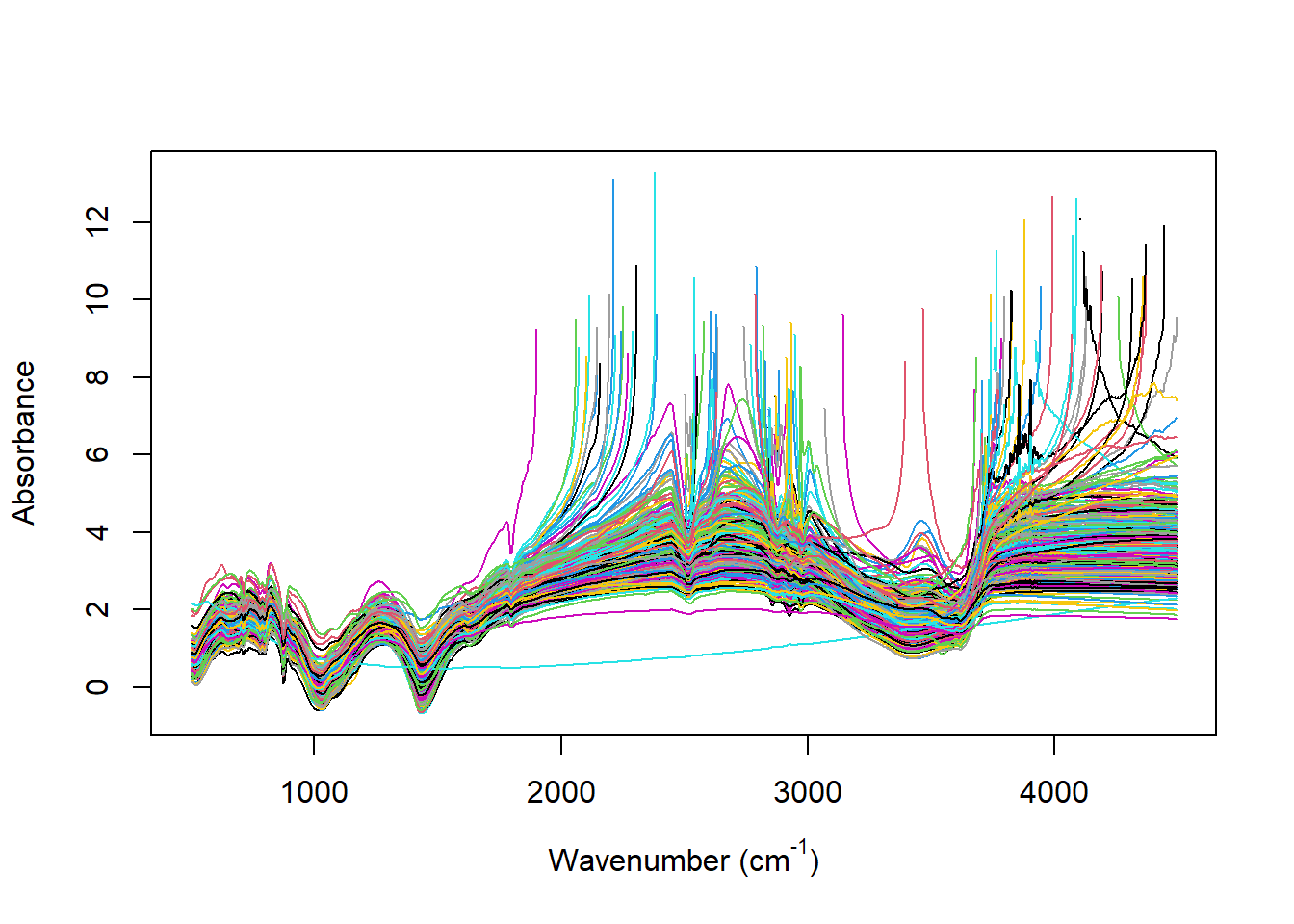
(#fig:plot wawenumber abso)Absorbance spectra in wavenumber.
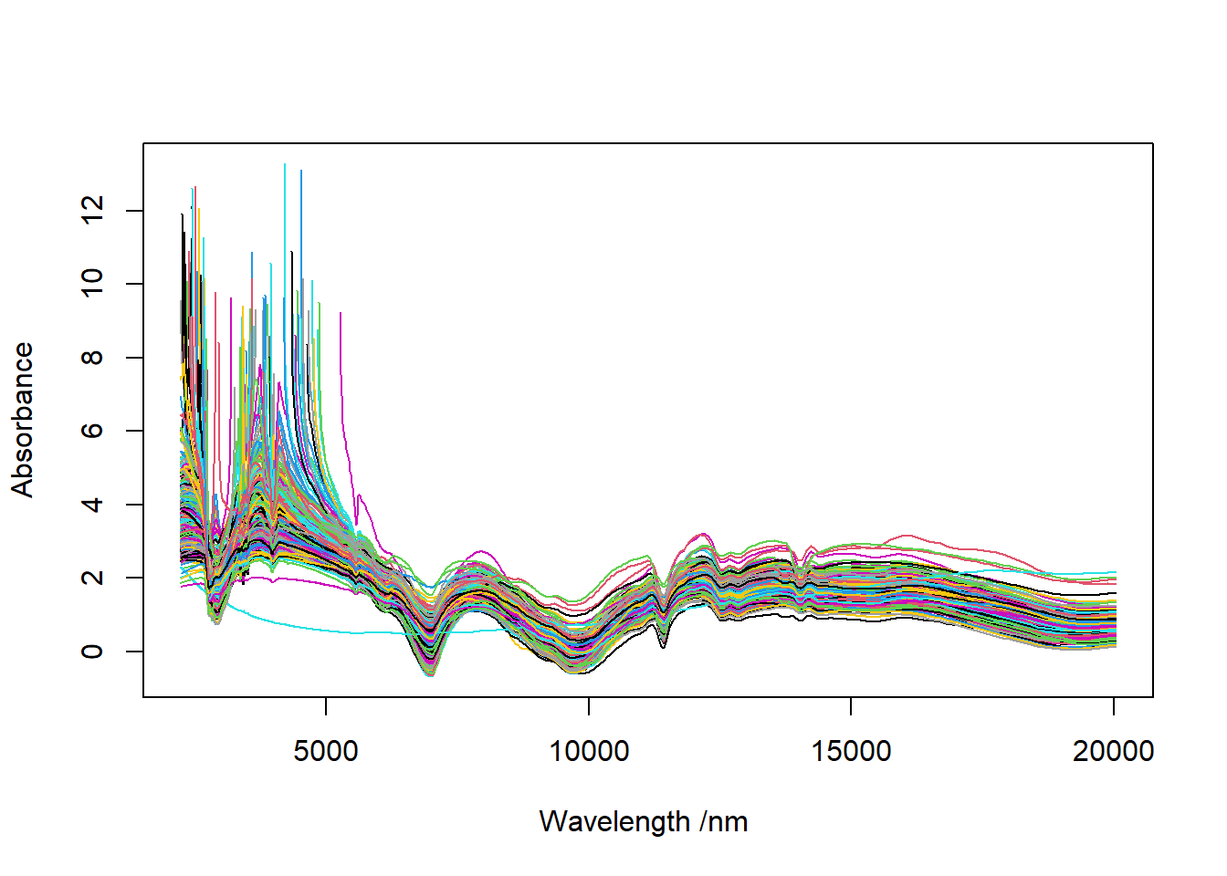
(#fig:plot wawelength abso)Absorbance spectra in wavelength.
4.5.2 The spectra in reflectance
# 4.2 Plot the reflectance #####################################################
png("Soil spectra in wavenumbers reflectance.png", width = 297, height = 210, units = "mm", res = 300)
pdf("Soil spectra in wavenumbers reflectance.pdf", width = 10*2, height = 6*2)

matplot(x = colnames(IRSpectra$wn), y = t(IRSpectra$wn),
        xlab = expression(paste("Wavenumber ", "(cm"^"-1", ")")),
        ylab = "Reflectance",
        type = "l",   #"l" = ligne
        lty = 1,
        col = 1:nrow(IRSpectra$wn))
dev.off()


png("Soil spectra in wavelength reflectance.png", width = 297, height = 210, units = "mm", res = 300)
pdf("Soil spectra in wavelength reflectance.pdf", width = 10*2, height = 6*2)

matplot(x = colnames(IRSpectra$wl), y = t(IRSpectra$wl),
        xlab = "Wavelength /nm ",
        ylab = "Reflectance",
        type = "l",   #"l" = ligne
        lty = 1,
        col = 1:nrow(IRSpectra$wl))
dev.off()
(#fig:plot wavenumber reflect)Reflectance spectra in wavenumber.
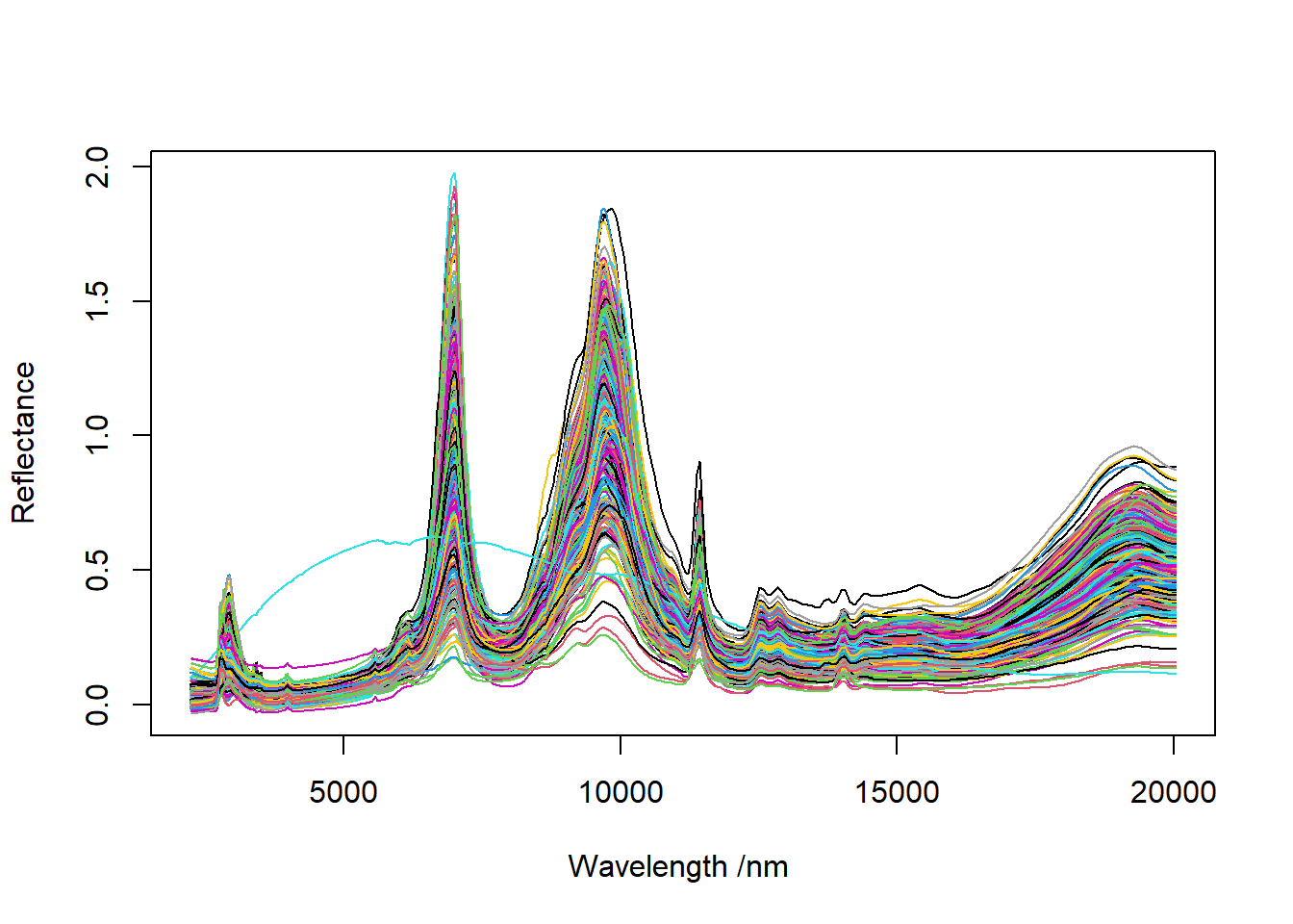
(#fig:plot wavelength reflect)Reflectance spectra in wavelength.
4.6 Kennard Stone sampling
The Kennard stone sampling is used to select a wide range of a population that will represent the diversity of the individuals (Kennard and Stone 1969). This sampling strategy has proven to be efficient in the soils spectrometry context (Ramirez-Lopez et al. 2014). We selected different numbers of samples for each depth increment with an over-representation of the topsoil (0 - 10 cm). All the samples from 2017 - 2018 were analysed, so no sampling strategy has been applied to them.
| Depth (cm) | Year | Number |
|---|---|---|
| 0 - 10 | 2022 | 30 |
| 10 - 30 | 2022 | 5 |
| 30 - 50 | 2022 | 5 |
| 50 - 70 | 2022 | 5 |
| 70 - 100 | 2022 | 5 |
| 0 - 10 | 2023 | 10 |
| 10 - 30 | 2023 | 4 |
| 30 - 50 | 2023 | 6 |
| 50 - 70 | 2023 | 6 |
| 70 - 100 | 2023 | 3 |
In the selection of samples, you can choose the year and depth increment. Here, we show a selection for the 2022 campaign at 0 - 10 cm depth. The table Samples_info use the information collected during the field campaign and the Field_observations file. The different entries are:
- Lab_ID Laboratory number gave at the samples when enter into Tübingen Soil Science and Geomrophology laboratory inventory.
- Site_name the site’s name according to the CLHS sampling.
- Depth_cm depth increment of the sampling (0 - 10 - 30 - 50 - 70 - 100 cm).
- X_WGS84 longitude in WGS84 (epsg:4326), measured from Garmin, GPSMAP 60Cx with ± 10 - 3 m accuracy (depending of satellite coverage).
- Y_WGS84 latitude in WGS84 (epsg:4326), measured from Garmin, GPSMAP 60Cx with ± 10 - 3 m accuracy (depending of satellite coverage).
# 05 Kennard Stone sampling ----------------------------------------------------
# 5.1 Select the samples #######################################################

Samples_info <- read_delim("./data/Samples_info.csv", delim = ";")
selection <- Samples_info[Samples_info$Depth_cm == "0_10" & grepl("B07_2022", Samples_info$Site_name), ] # You can select the year and the depth

# Select the samples to analyse
MIRsample <- MIRspec_wl[rownames(MIRspec_wl) %in% selection$Lab_ID,]

# 5.2 Run the sampling #########################################################
sample <- kenStone(MIRsample, k = 30, metric = "euclid") # Make samples with Kennard Stone in euclidian distance

MIRsample <- MIRsample[sample$model,]
MIRsample <- row.names(MIRsample)
write.table(MIRsample, "./export/samples/B07_2022 Samples 0 - 10 cm.txt", dec = ".", sep = ";", row.names = FALSE, col.names = FALSE, append = FALSE)