8 Soil depth mapping
8.1 Introduction
8.1.1 Purpose
This document is meant to present the methodology we used for soil depth mapping. Our data are based on the sampling campaigns 2022 - 2023 and additional remote sensing observation for bare rock formations. We based our approach on Liu et al. (2022) and added small modifications.
8.1.2 Covariates
All the data listed below are available freely online excepted for the digitized maps (Geology).
| Name/ID | Original resolution (m) | Type/Unit |
|---|---|---|
| Aspect/TE.1 | 30 | Radians |
| DEM/TE.5 | 30 | Meters |
| General curvature/TE.7 | 30 | - |
| MrRTF/TE.8 | 30 | - |
| MrVBF/TE.9 | 30 | - |
| Plan curvature/TE.12 | 30 | - |
| Profile curvature/TE.14 | 30 | - |
| Slope/TE.16 | 30 | Radians |
| TPI/TE.21 | 30 | - |
| Landsat 5 B2/LA5.1 | 30 | 0.52 - 0.60 µm |
| Landsat 5 B3/LA5.2 | 30 | 0.63 - 0.69 µm |
| Landsat 5 B4/LA5.3 | 30 | 0.76 - 0.90 µm |
| Landsat 5 B7/LA5.4 | 30 | 2.08 - 2.35 µm |
| Landsat 5 NDVI/LA5.5 | 30 | - |
| Landsat 5 NDWI/LA5.6 | 30 | - |
| LST Apr-May/LST.1 | 1000 | Kelvin |
| LST Feb-Mar/LST.2 | 1000 | Kelvin |
| LST Jun-Jul/LST.3 | 1000 | Kelvin |
| LST Oct-Nov/LST.4 | 1000 | Kelvin |
| Geology/OT.2 | 1 : 250 000 | Lithology |
| Landuse/OT.4 | 10 | Landuse class |
| PET sum/OT.5 | 750 | mm |
| Prec. sum/OT.6 | 1000 | mm |
| SRAD sum/OT.7 | 1000 | MJ m\(^{-2}\) |
| Wind sum/OT.9 | 1000 | m s\(^{-1}\) |
| Temp avg/OT.10 | 1000 | °C |
8.1.2.1 Terrain
All terrain covariates were computed the same way as in the previous chapter.
8.1.2.2 Remote sensing images and indexes
The Landsat 5 images were collected via a Google Earth Engine script on a period covering 1990 - 2010, the median of the composite image from Collection 2 Tier 1 TOA was used. The land surface temperature (LST) were computed also on Google Earth Engine with a time covering from 2012 to 2016 from the Suomi National Polar-Orbiting satellite. We took the average of each period: February - Mars, April - May, June - July and October November from the VIIRS instrument. The javascript codes for scraping these images are available in the supplementary file inside the “8 - Soil depth/code” folder. We computed the following indexes: Normalized Difference Vegetation Index (NDVI) (McFeeters 1996) and Normalized Difference Water Index (NDWI) (Rouse et al. 1974).
\[ NDVI = (NIR - Red) / (NIR + Red) \]
\[ NDWI = (Green - NIR) / (Green + NIR) \]
import ee
import geemap
import rasterio
from rasterio.features import shapes
import geopandas as gpd
from shapely.geometry import mapping
from shapely.geometry import shape
import os
from pydrive.auth import GoogleAuth
from pydrive.drive import GoogleDrive

ee.Authenticate()
ee.Initialize()

# Local file
raster_path = r".\data\Large_grid.tif"
with rasterio.open(raster_path) as src:
    image = src.read(1)
    mask = image > 0
    results = (
        {'properties': {'value': v}, 'geometry': s}
        for i, (s, v) in enumerate(
            shapes(image, mask=mask, transform=src.transform))
    )

# Convert in GeoDataFrame
geoms = list(results)
gdf = gpd.GeoDataFrame.from_features(geoms)

# Create a polygon and gee object
aoi_poly = gdf.union_all()
aoi = ee.Geometry(mapping(aoi_poly))

Map = geemap.Map()
Map.centerObject(aoi, 8)
Map.addLayer(aoi, {}, "AOI")
Map

def maskL5clouds(image):
    qa = image.select('QA_PIXEL')

    cloudBit        = 1 << 3
    cloudShadowBit  = 1 << 4

    mask = (qa.bitwiseAnd(cloudBit).eq(0)
            .And(qa.bitwiseAnd(cloudShadowBit).eq(0)))
    return image.updateMask(mask)

dataset = (
    ee.ImageCollection("LANDSAT/LT05/C02/T1_TOA")
    .filterDate("1990-01-01", "2010-12-31")  # period
    .map(maskL5clouds)
)

# Median
L5_composite = dataset.median().clip(aoi)

dataset = (
    ee.ImageCollection("NOAA/VIIRS/001/VNP21A1D")
    .filterDate("2016-02-01", "2016-03-30")  # period
)

# Median
LST_01_composite = dataset.median()
LST_01 = LST_01_composite.select('LST_1KM').clip(aoi)

dataset = (
    ee.ImageCollection("NOAA/VIIRS/001/VNP21A1D")
    .filterDate("2016-04-01", "2016-05-30")  # period
)

# Median
LST_02_composite = dataset.median().clip(aoi)
LST_02 = LST_02_composite.select('LST_1KM').clip(aoi)

dataset = (
    ee.ImageCollection("NOAA/VIIRS/001/VNP21A1D")
    .filterDate("2016-06-01", "2016-07-30")  # period
)

# Median
LST_03_composite = dataset.median().clip(aoi)
LST_03 = LST_03_composite.select('LST_1KM').clip(aoi)

dataset = (
    ee.ImageCollection("NOAA/VIIRS/001/VNP21A1D")
    .filterDate("2016-10-01", "2016-11-30")  # period
)

# Median
LST_04_composite = dataset.median().clip(aoi)
LST_04 = LST_04_composite.select('LST_1KM').clip(aoi)

geemap.ee_export_image(
    LST_01,
    filename=r".\data\NPP\LST_feb_mar_raw.tif",
    scale=1000,
    region=aoi,
    crs="EPSG:32638"
)

geemap.ee_export_image(
    LST_02,
    filename=r".\data\NPP\LST_apr_may_raw.tif",
    scale=1000,
    region=aoi,
    crs="EPSG:32638"
)

geemap.ee_export_image(
    LST_03,
    filename=r".\data\NPP\LST_jun_jul_raw.tif",
    scale=1000,
    region=aoi,
    crs="EPSG:32638"
)

geemap.ee_export_image(
    LST_04,
    filename=r".\data\NPP\LST_oct_nov_raw.tif",
    scale=1000,
    region=aoi,
    crs="EPSG:32638"
)

L5_bands = ['B2', 'B3', 'B4', 'B7']

for band in L5_bands:
    task = ee.batch.Export.image.toDrive(
        image=L5_composite.select([band]),
        description = f"Landsat5_{band}_2010_MedianComposite",
        scale = 30,
        region = aoi,
        crs = 'EPSG:32638',
        folder = 'GoogleEarthEngine',
        maxPixels = 1e13
    )
    task.start()
8.1.3 Soil depths
The soil depths of the 122 soil profiles were measured during the field campaign and can be found found online at: https://doi.org/10.1594/PANGAEA.973714. Additional 25 site with no soil (or zero value to soil depth), were added after looking at Bing and Google earth satellite image. We only selected bare rock formation for these sites.
8.2 Soil depth mapping prediction
8.2.1 Preparation of the environment
# 0 Environment setup ##########################################################

# 0.1 Prepare environment ======================================================

# Folder check
getwd()

# Set folder direction
setwd()

# Clean up workspace
rm(list = ls(all.names = TRUE))

# 0.2 Install packages =========================================================

install.packages("pacman")        #Install and load the "pacman" package (allow easier download of packages)
library(pacman)

pacman::p_load(ggplot2, terra, mapview, sf, dplyr, corrplot, viridis, rsample, caret, parsnip, tmap, geodata, googledrive, ggnewscale,
               parallel, doParallel, cli, patchwork, quantregForest, ncdf4, wesanderson, cblindplot, grid, gridExtra, ggspatial, cowplot)

# 0.3 Show session infos =======================================================

sessionInfo()
8.2.2 Preparation of the data
All raster were sampled to 30 x 30 m tiles to match the DEM. We used bilinear method excepted for the discrete maps (geology) where we used ngb resampling.
# 01 Import data sets ##########################################################
# 01.1 Import soils depths =====================================================
# From the data accessible at the https://doi.org/10.1594/PANGAEA.973714
# We added 25 NULL results from bare rock point spoted in remote sensing images
depth <- read.csv ("./data/Soil_depth.csv", sep=";")
depth$Depth <- as.numeric(depth$Depth)
# 01.2 Plot the depth information ==============================================
# Short overview of the values
head(depth)
# Histogram of the values
ggplot(depth, aes(x = Depth)) +
geom_histogram(breaks = seq(0, 100, by = 10), alpha = 0.5, fill = 'steelblue', color = 'black') +
labs(title ="Number of sample for each soil depth in cm", x = "Depth in cm", y = "Number of samples") +
xlim(0, 100) +
theme_minimal() +
theme(plot.title = element_text(hjust = 0.5))
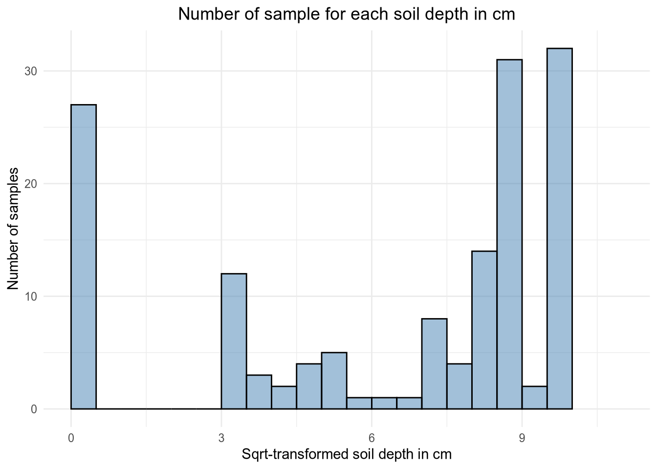
# 01.3 Transform and plot the data =============================================
depth$sqrt <- sqrt(depth$Depth)
# Histogram of the sqrt values
ggplot(depth, aes(x = sqrt)) +
geom_histogram(breaks = seq(0, 10, by = 0.5), alpha = 0.5, fill = 'steelblue', color = 'black') +
labs(title ="Number of sample for each soil depth in cm", x = "Sqrt-transformed soil depth in cm", y = "Number of samples") +
xlim(0, 11) +
theme_minimal() +
theme(plot.title = element_text(hjust = 0.5))
# 01.4 Plot the depth spatial information ======================================
# Create a spatial dataframe with WGS84 UTM 38 N cordinates
sp_df <- st_as_sf(depth, coords = c("X", "Y"), crs = 32638)
# Plot the values of depth regarding the elevation
mapview(sp_df, zcol = "Depth", legend =TRUE, map.types ="Esri.WorldShadedRelief") ## X Y Site.Name Depth
## 1 287940.2 4095202 B07_2022_001 100
## 2 286917.0 4104485 B07_2022_002 65
## 3 280594.1 4090376 B07_2022_003 40
## 4 275039.6 4097134 B07_2022_004 80
## 5 289512.9 4086706 B07_2022_006 80
## 6 287922.6 4092158 B07_2022_007 0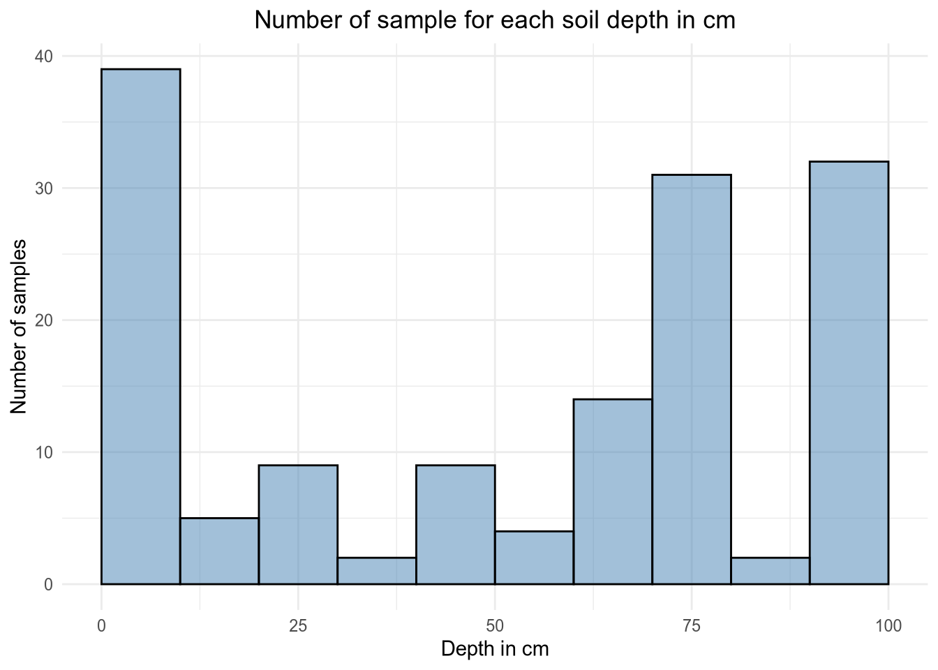
# 02 Prepare the covariates ####################################################

# 02.1 Import background layers ================================================
DEM <- rast("../07 - DSM/data/Others/DEM.tif")

# 02.2 Import from Google Drive ================================================
drive_auth()
files <- drive_ls()

# Import Landsat 5
file <- files[grepl("Landsat5", files$name), ]
for (i in 1:nrow(file)) {
  drive_download(
    as_id(file$id[[i]]),
    path = paste0("./data/Landsat/Raw_",file[[1]][[i]]),
    overwrite = TRUE)
}

# 02.3 Resize NPP and Landsat data =============================================
NPP_raw <- list.files("./data/NPP", pattern = "*_raw", full.names = TRUE)
NPP_raw  <- rast(NPP_raw)

for (i in 1:nlyr(NPP_raw)) {
  r <-resample(NPP_raw[[i]], DEM, method = "bilinear")
  r <- crop(r, DEM)
  names(r) <- gsub("_raw", "", names(r))
  writeRaster(r, paste0("./data/NPP/",names(r),".tif"), overwrite=T)
}

all_files <- list.files("./data/NPP", full.names = TRUE)
NPP <- rast(all_files[!grepl("raw", all_files)])

Landsat <- rast(list.files("./data/Landsat/",  pattern = "*Raw", full.names = TRUE))
Landsat_names <- list.files("./data/Landsat/",pattern = "*Raw", full.names = FALSE)

patterns  <- c("B2", "B3", "B4", "B7")
replacers <- c("blue", "green", "red", "NIR")

for (i in seq_along(patterns)) {
  Landsat_names <- gsub(patterns[i], replacers[i], Landsat_names)
}
names(Landsat) <- gsub("\\.tif$", "", Landsat_names)
names(Landsat) <- gsub("Raw_", "", names(Landsat))
names(Landsat) <- gsub("_2010_MedianComposite", "", names(Landsat))

Landsat$Landsat5_NDWI <- (Landsat$Landsat5_green - Landsat$Landsat5_NIR)/(Landsat$Landsat5_green + Landsat$Landsat5_NIR)
Landsat$Landsat5_NDVI <- (Landsat$Landsat5_NIR - Landsat$Landsat5_red)/(Landsat$Landsat5_NIR +  Landsat$Landsat5_red)

for (i in 1:nlyr(Landsat)) {
  r <-resample(Landsat[[i]], DEM, method = "bilinear")
  r <- crop(r, DEM)
  writeRaster(r, paste0("./data/Landsat/",names(r),".tif"), overwrite=T)
}

all_files <- list.files("./data/Landsat/",  full.names = TRUE)
Landsat <- rast(all_files[!grepl("Raw", all_files)])

# 02.4 Import other covariates  ================================================
Others <- list.files("../07 - DSM/data/Others/", full.names = TRUE)
Others <- rast(Others[c(4,6,8,10,11,12,13)])

Others_names <- list.files("../07 - DSM/data/Others/", full.names = FALSE)
Others_names <- Others_names[c(4,6,8,10,11,12,13)]
Others_names <- gsub("\\.tif$", "", Others_names)

names(Others) <- Others_names

Terrain <- list.files("../07 - DSM/SAGA/", pattern = "*sg-grd-z" , full.names = TRUE)
Terrain <- rast(Terrain[c(1,6,12,16,17,20,22,24,29)])
names(Terrain)[names(Terrain) == "DEM [no sinks] [Smoothed]"] <- "DEM"

DSM_cov_name <- read.table("../07 - DSM/data/Covariates_names_DSM.txt")

df_names <- data.frame()
for (i in 1:length(names(Terrain))) {
  col_name <- names(Terrain)[i]
  if (col_name %in% DSM_cov_name$V2) {
    transformed_name <- DSM_cov_name$V1[DSM_cov_name$V2 == col_name]
  } else {
    transformed_name <- paste0("TE.25")
  }
  df_names[i,1] <- transformed_name
  df_names[i,2] <- names(Terrain)[i]
}

t <- nrow(df_names)
for (i in 1:length(names(Landsat))) {
  c <- paste0("LA5.",i)
  df_names[i+t,1] <- c
  df_names[i+t,2] <- names(Landsat)[i]
}

t <- nrow(df_names)
for (i in 1:length(names(NPP))) {
  c <- paste0("NPP.",i)
  df_names[i+t,1] <- c
  df_names[i+t,2] <- names(NPP)[i]
}

t <- nrow(df_names)
for (i in 1:length(names(Others))) {
  col_name <- names(Others)[i]
  if (col_name %in% DSM_cov_name$V2) {
    transformed_name <- DSM_cov_name$V1[DSM_cov_name$V2 == col_name]
  } else {
    transformed_name <- "OT.10"
  }
  df_names[i+t,1] <- transformed_name
  df_names[i+t,2] <- names(Others)[i]
}

write.table(df_names,"./data/Covariates_names_soil_depth.txt")
all_cov_name <- rbind(DSM_cov_name, df_names)
all_cov_name <- distinct(all_cov_name)
x <- c(Terrain, Landsat, NPP, Others)
names(x) <- df_names[,1]

reduce <- aggregate(x, fact=10, fun=modal)
writeRaster(reduce, "./data/Stack_layers_DSM_reduce.tif", overwrite = TRUE)

plot(reduce)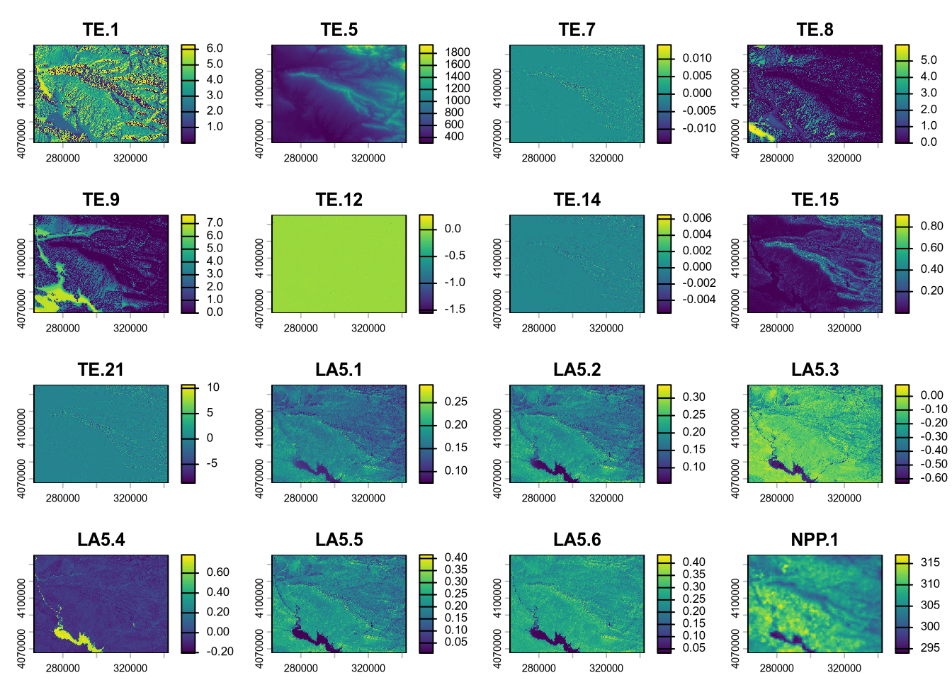
(#fig:script plot cov depth hide-1)Covariates from soil depth model.
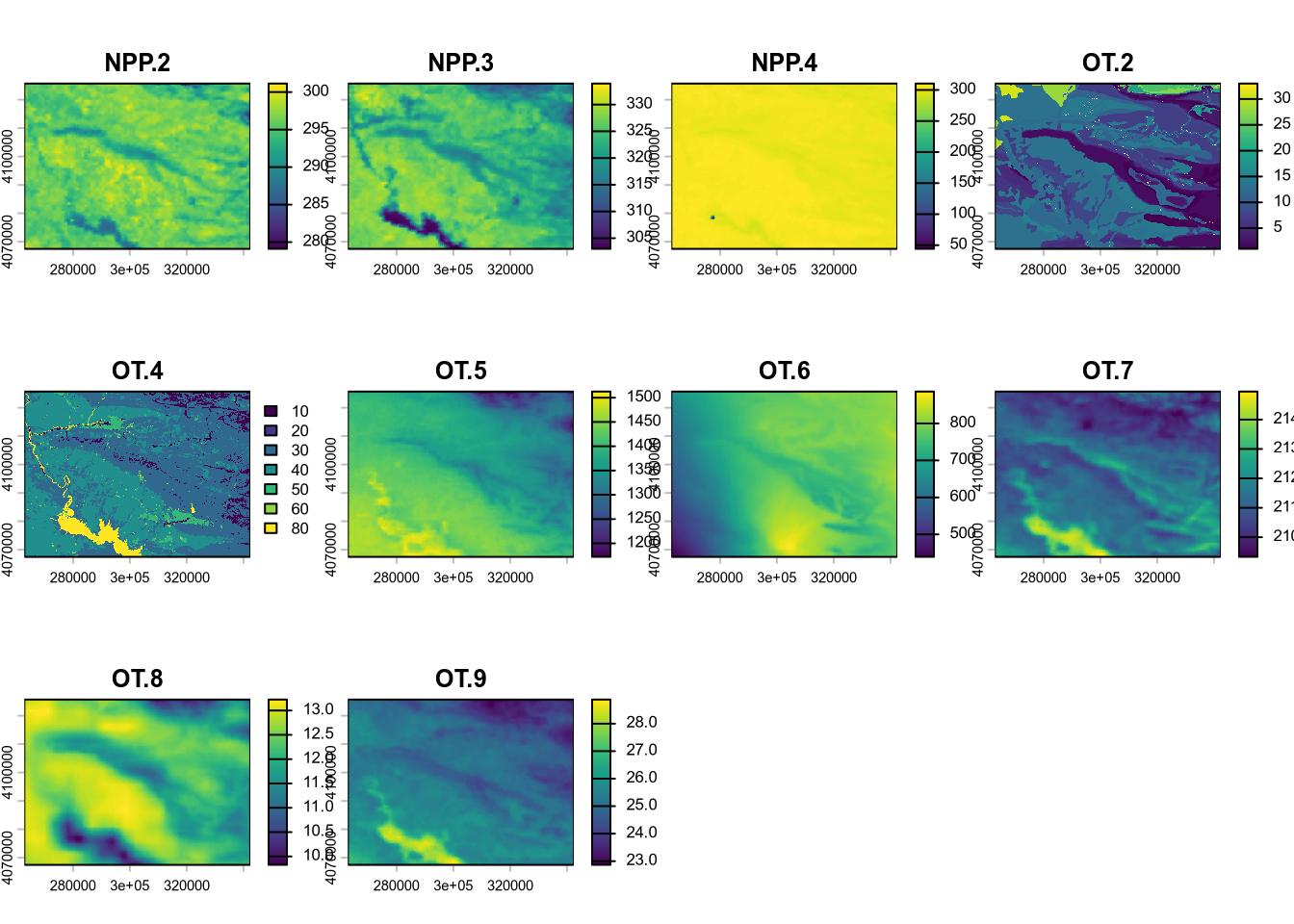
(#fig:script plot cov depth hide-2)Covariates from soil depth model.
# 02.5 Extract the values ======================================================

# Extract the values of each band for the sampling location
df_cov <- extract(x, sp_df, method='simple')

# 02.6 Save the data ===========================================================

# Create a csv out of it
writeRaster(x, "./data/Stack_layers_soil_depth.tif", overwrite = TRUE)
write.csv(data.frame(df_cov[,-c(1)]), "./data/df_cov_soil_depth.csv")

# 03 Check the data ############################################################

# 03.1 Import the data and merge ===============================================
Covdfgis    <- read.csv("./data/df_cov_soil_depth.csv")
ID    <- 1:nrow(Covdfgis)
SoilCov <- cbind(ID, depth, Covdfgis[,-c(1)])

#Check the data
names(SoilCov)
str(SoilCov)

# 03.2 Check and prepare the data ==============================================

# Prepare data for ML modelling
SoilCovML <- SoilCov[,-c(1:6)]

# 03.3 Plot and export the correlation matrix ==================================
pdf("./export/Correlation.pdf",    # File name
    width = 20, height = 20,  # Width and height in inches
    bg = "white",          # Background color
    colormodel = "cmyk")   # Color model


# Correlation of the data
corrplot(cor(SoilCovML[,-c(20:21)]),  method = "color", col = viridis(200),
         type = "upper",
         addCoef.col = "black", # Add coefficient of correlation
         tl.col = "black", tl.srt = 45, # Text label color and rotation
         number.cex = 0.7, # Size of the text labels
         cl.cex = 0.7, # Size of the color legend text
         cl.lim = c(-1, 1)) # Color legend limits

dev.off()

save(SoilCov, file = "./export/save/Pre_process_soil_depth.RData")
rm(list=setdiff(ls(), c("SoilCov")))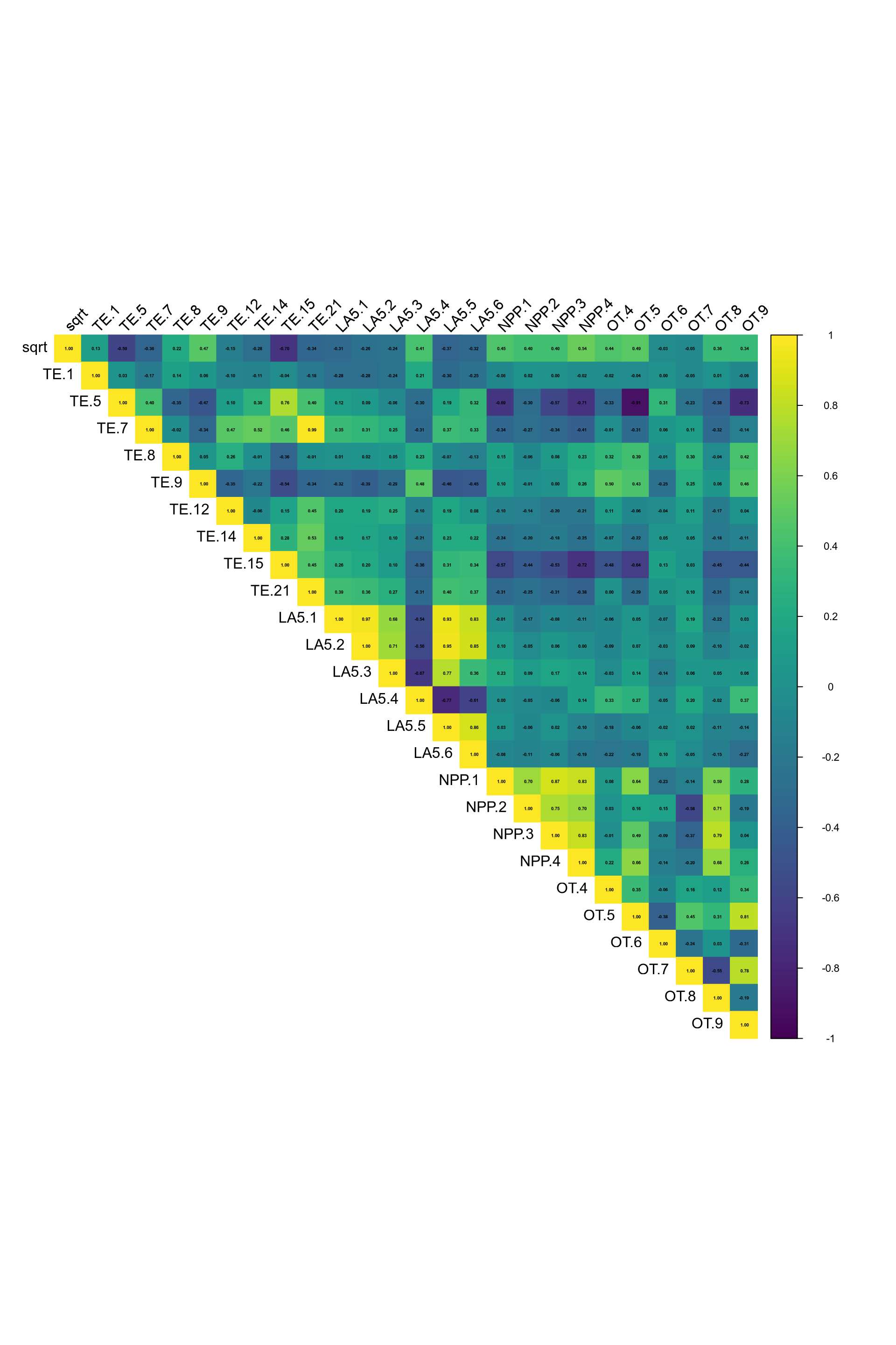
(#fig:depth corrplot hide)Auto-correlation plot soil depth covariates.
Regarding the correlation plot, the Landsat 5 bands and land surface temperature layers have correlation index over 0.75, as some transformed layers based on DEM (curvature, slope ,aspect …) and the solar radiation with wind.
8.2.3 Tune the model
The QRF model used is similar to the one for DSM.
# 04 Tune the model ############################################################
covariates <- rast("./data/Stack_layers_soil_depth.tif")

# 04.1 Prepare the data set and the models =====================================

#R Remove the site name and x, y columns
df_soilCov <- SoilCov[,c(1,5:length(SoilCov))]

# Set a random seed
set.seed(1070)

# Remove NZV (if any)
nzv <- nearZeroVar(df_soilCov[,4:length(df_soilCov)], saveMetrics = TRUE)
rownames(nzv)[nzv$nzv == TRUE]

# 04.2 Create the model train controls with cross-validation  ==================
source("../07 - DSM/script/QRF_models.R")

set.seed(1070)
TrainControl <- trainControl(method="repeatedcv", 10, 3, allowParallel = TRUE, savePredictions=TRUE, verboseIter = TRUE)

data <- df_soilCov[,3:length(df_soilCov)]

# 04.2 Run the model ===========================================================

start_time <- Sys.time()
qrf_model <- train(sqrt ~ ., data,
                   method = qrf_caret,
                   trControl = TrainControl,
                   metric = "RMSE",
                   tuneGrid = expand.grid(mtry = c(1:ncol(data-1)), nodesize = seq(1,21, by = 5)),
                   ntree = 500)

end_time <- Sys.time()
print(end_time - start_time)

# 04.3 Compute metrics =====================================================

best_params <- qrf_model$bestTune

pred_best <- qrf_model$pred %>%
  dplyr::filter(
    mtry == best_params$mtry,
    nodesize == best_params$nodesize
  )

pred_best$pred <- as.numeric(pred_best$pred)

metrics_by_best <- pred_best %>%
  group_by(Resample) %>%
  summarise(
    ME   = mean(pred^2 - obs^2, na.rm = TRUE),
    RMSE = sqrt(mean((pred^2 - obs^2)^2, na.rm = TRUE)),
    R2   = cor(pred^2, obs^2, use = "complete.obs")^2,
    PICP = mean(obs^2 >= pred.quantile..0.05^2 & obs^2 <= pred.quantile..0.95^2, na.rm = TRUE))

metrics_df <- as.data.frame(metrics_by_best)

metrics_summary <- metrics_df %>%
  summarise(
    ME_mean   = mean(ME),
    RMSE_mean = mean(RMSE),
    R2_mean   = mean(R2),
    PICP_mean = mean(PICP),
    ME_sd     = sd(ME),
    RMSE_sd   = sd(RMSE),
    R2_sd     = sd(R2),
    PICP_sd   = sd(PICP)
  )

print(metrics_summary)


png("./export/Models_tuning_parameters_for_soil_depth.png",
    width = 600, height = 500)
plot(qrf_model, main = "QRF tuning parameters for soil depth")
dev.off()

pdf("./export/Models_tuning_parameters_for_soil_depth.pdf",
    width = 6, height = 5,
    bg = "white")
plot(qrf_model, main = "QRF tuning parameters for soil depth")
dev.off()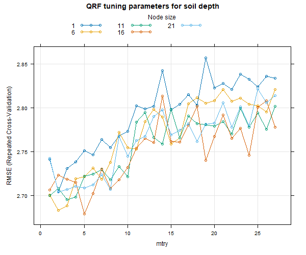
8.2.4 Variables imortance
# 04.4 Plot variable importance ================================================

var_importance <- varImp(qrf_model, scale = TRUE)
importance_df <- as.data.frame(var_importance$importance)
importance_df$Variable <- rownames(importance_df)

AvgVarImportance <- importance_df %>%
  group_by(Variable) %>%
  summarise(importance_df = mean(Overall, na.rm = TRUE)) %>%
  arrange(desc(importance_df))

# Select top 20 variables
Top20Var <- AvgVarImportance %>%
  top_n(20, wt = importance_df)


AllVarImportanceTop20 <- AvgVarImportance %>%
  filter(Variable %in% Top20Var$Variable)

colnames(AllVarImportanceTop20) <- c("Covariable", "Importance")

VarPlot <- ggplot(AllVarImportanceTop20, aes(x = reorder(Covariable, Importance), y = Importance)) +
  geom_bar(stat = "identity", position = "dodge", fill = "lightblue") +
  coord_flip() +
  labs(title = "Top 20 covariates influence for soil depth",
       x = "Covariates",
       y = "Importance") +
  theme_minimal() +
  theme(plot.title = element_text(hjust = 0.5))


png("./export/Variables_importance_for_soil_depth.png",
    width = 600, height = 500)
plot(VarPlot)
dev.off()

pdf("./export/Variables_importance_for_soil_depth.pdf",
    width = 6, height = 5,
    bg = "white")
plot(VarPlot)
dev.off()

write.csv(data.frame(metrics_summary), "./export/Models_metrics_soil_depth.csv")
write.csv(AllVarImportanceTop20, "./export/Variable_importance_soil_depth.csv")

# 04.5 Save the model and train and test sets ==================================
save(qrf_model, file = "./export/save/Model_soil_depth.RData")
rm(list = ls())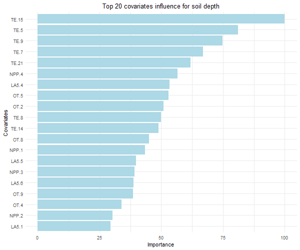
8.2.5 Model evaluation
We used four metrics to evaluate the model:
- ME = Bias with the mean error.
- RMSE = Root mean square error.
- R\(^2\) = Coefficient of determination, also called rsquared.
- PICP = Prediction interval coverage probability set at 90% interval
\[ \\[0.5cm] ME = \frac{1}{n} \sum_{i=n}^{n}(\hat{y}_i - y_i) \]
Where: \(n\) is the number of observations, \(y_i\) the observed value for \(i\), and \(\hat{y}_i\) the predicted value for \(i\).
\[ \\[0.5cm] RMSE = \sqrt{\frac{\sum_{i=1}^{n}(y_i - \hat{y}_i)^2}{N}} \]
Where: \(n\) is the number of observations, \(y_i\) the observed value for \(i\), and \(\hat{y}_i\) the predicted value for \(i\).
\[ \\[0.5cm] R^2 = 1 - \frac{\sum_{i=1}^{n}(y_i - \hat{y}_i)^2}{\sum_{i=1}^{n}(y_i - \bar{y}_i)^2} \]
Where: \(y_i\) the observed value for \(i\), \(\hat{y}_i\) the predicted value for \(i\), and \(\bar{y}\) is the mean of observed values.
\[ \\[0.5cm] PICP = \frac{1}{v} ~ count ~ j \\ j = PL^{L}_{j} \leq t_j \leq PL^{U}_{j} \]
Where: \(v\) is the number of observations, \(obs_i\) is the observed value for \(i\), \(PL^{L}_{i}\) is the lower prediction limit for \(i\), and \(PL^{U}_{i}\) is the upper prediction limit for \(i\).
##    ME_mean RMSE_mean   R2_mean PICP_mean    ME_sd  RMSE_sd     R2_sd    PICP_sd
## 1 3.269185  30.75852 0.3908253 0.9887103 6.232449 5.033474 0.1634309 0.02571429
8.2.6 Mapping the soil depth of the area
Due to the highly detailed data we had to split the prediction into different blocks. This process allows the computer to run separately each prediction.
The uncertainty of the model is based on the following equation from Yan et al. (2018).
\[ \\[0.5cm] Uncertainty = \frac{Qp ~ 0.95- Qp ~ 0.05}{Qp ~ 0.5} \]
# 05 Predict the map ###########################################################
# 05.1 Import the previous data ================================================
load(file = "./export/save/Model_soil_depth.RData")
covariates <- rast("./data/Stack_layers_soil_depth.tif")

cov_df <- as.data.frame(covariates, xy = TRUE)
cov_df[is.infinite(as.matrix(cov_df))] <- NA
cov_df <- na.omit(cov_df)
cov_names <- names(covariates)

n_blocks <- 10
cov_df$block <- cut(1:nrow(cov_df), breaks = n_blocks, labels = FALSE)
cov_df_blocks <- split(cov_df, cov_df$block)

predicted_blocks <- list()

cli_progress_bar(
  format = "Prediction depth {cli::pb_bar} {cli::pb_percent} [{cli::pb_current}/{cli::pb_total}] | \ ETA: {cli::pb_eta} - Time elapsed: {cli::pb_elapsed_clock}",
  total = n_blocks,
  clear = FALSE)

cl <- makeCluster(6)
registerDoParallel(cl)

# Create a loop for blocks
for (i in 1:10) {
  block <- cov_df_blocks[[i]][,cov_names]
  prediction <- predict(qrf_model$finalModel, newdata = block, what = c(0.05, 0.5, 0.95))^2
  predicted_df <- cov_df_blocks[[i]][,c(1:2)]
  predicted_df$median <- prediction[,2]
  predicted_df$min <- prediction[,1]
  predicted_df$max <- prediction[,3]
  predicted_blocks[[i]] <- predicted_df
  cli_progress_update()
}
cli_progress_done()

predicted_rast <- do.call(rbind,predicted_blocks)
predicted_rast <- rast(predicted_rast, type ="xyz")
crs(predicted_rast) <- crs(rast)
predicted_rast$uncertainty <- (predicted_rast$max - predicted_rast$min) /predicted_rast$median

writeRaster(predicted_rast, "./export/Prediction_depth.tif", overwrite=TRUE)
stopCluster(cl)
rm(list = ls())
8.3 Visualisations and exports
8.3.1 Basic visualisations
# 06 Visualisation of the prediction ###########################################
# 06.1 Plot the depth maps =====================================================
load(file = "./export/save/Pre_process_soil_depth.RData")
raster <- rast("./export/Prediction_depth.tif")
crs(raster) <- "EPSG:32638"
survey <- st_read("../07 - DSM/data/Survey_Area.gpkg", layer = "Survey_Area")
sp_df <- st_as_sf(SoilCov, coords = c("X", "Y"), crs = "EPSG:32638")

summary(raster)

# Remove the NA
for(i in 1:nlyr(raster)) {
  name <- names(raster[[i]])
  raster[[name]] <- focal(raster[[i]],
                       w = 3,
                       fun = mean,
                       na.rm = TRUE,
                       na.policy = "only")
}

summary(raster)

predicted_raster_resize <- aggregate(raster, fact=5, fun=mean)

# Plot continuous values of the map
mapview(predicted_raster_resize$median, at = seq(0,100,20), legend = TRUE, layer.name = "Soil depth prediction (cm)",col.regions = wes_palettes$Zissou1Continuous) +
  mapview(sp_df, zcol = "Depth", at = seq(0,100,20),  legend = TRUE, layer.name = "Soil samples depth (cm)", col.regions = wes_palettes$Zissou1Continuous)

mapview(predicted_raster_resize$uncertainty,  at = seq(0,14,2), legend = TRUE)
## Reading layer `Survey_Area' from data source
## `/home/mathias/Bureau/Traitement/07 - DSM/data/Survey_Area.gpkg'
## using driver `GPKG'
## Simple feature collection with 1 feature and 2 fields
## Geometry type: MULTIPOLYGON
## Dimension: XY
## Bounding box: xmin: 264456.8 ymin: 4070092 xmax: 338528.5 ymax: 4122549
## Projected CRS: WGS 84 / UTM zone 38N## Warning: [summary] used a sample## median min max uncertainty
## Min. : 0.00 Min. : 0.000 Min. : 0.00 Min. : 0.7
## 1st Qu.: 10.00 1st Qu.: 0.000 1st Qu.:100.00 1st Qu.: 1.2
## Median : 50.00 Median : 0.000 Median :100.00 Median : 1.8
## Mean : 46.79 Mean : 3.565 Mean : 92.86 Mean : Inf
## 3rd Qu.: 75.00 3rd Qu.:10.000 3rd Qu.:100.00 3rd Qu.:10.0
## Max. :100.00 Max. :34.741 Max. :100.00 Max. : Inf
## NA's :5 NA's :5 NA's :5 NA's :401## Warning: [summary] used a sample## median min max uncertainty
## Min. : 0.00 Min. : 0.000 Min. : 0.00 Min. : 0.700
## 1st Qu.: 10.00 1st Qu.: 0.000 1st Qu.:100.00 1st Qu.: 1.200
## Median : 50.00 Median : 0.000 Median :100.00 Median : 1.822
## Mean : 46.78 Mean : 3.565 Mean : 92.86 Mean : Inf
## 3rd Qu.: 75.00 3rd Qu.:10.000 3rd Qu.:100.00 3rd Qu.:10.000
## Max. :100.00 Max. :34.741 Max. :100.00 Max. : Inf
## NA's :87\(\\[0.5cm]\)
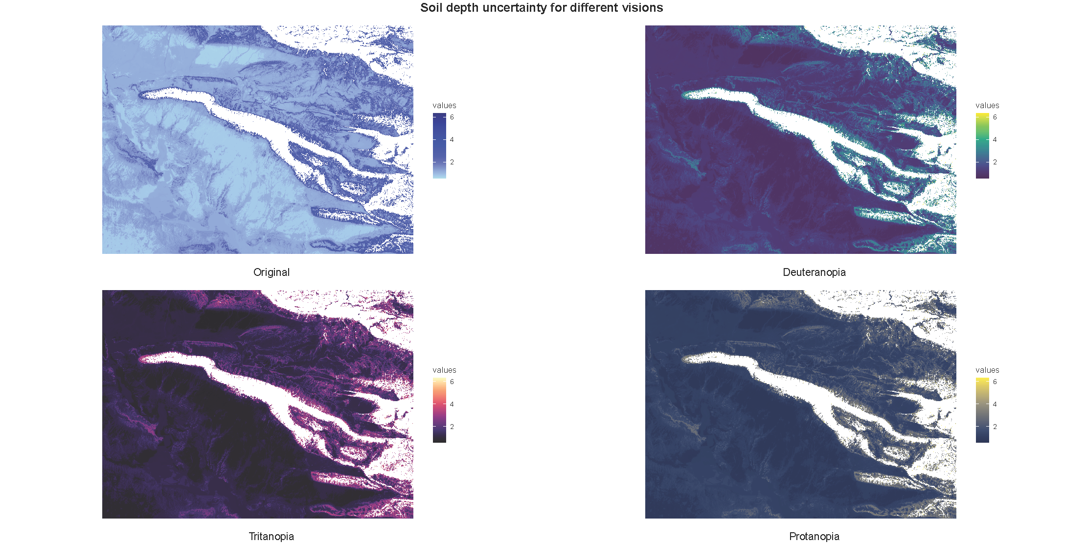
8.3.2 Colorblind visualisations
# 06.2 Visualise for colorblind ================================================

wes_palette_hcl <- function(palette_name, n = 7) {
  wes_colors <- wes_palette(palette_name, n = n, type = "continuous")
  hex_colors <- as.character(wes_colors)
  return(hex_colors)
}

palette_wes <- rev(wes_palette_hcl("Zissou1", n = 7))
palette_blue <- colorRampPalette(c("lightblue", "blue", "darkblue"))(7)

# Predictions
gg1 <- cblind.plot(predicted_raster_resize$median, cvd = palette_wes)
gg2 <- cblind.plot(predicted_raster_resize$median, cvd = "deuteranopia")
gg3 <- cblind.plot(predicted_raster_resize$median, cvd = "tritanopia")
gg4 <- cblind.plot(predicted_raster_resize$median, cvd = "protanopia")

grid <- grid.arrange(
  arrangeGrob(gg1, bottom = textGrob("Original", gp = gpar(fontsize = 14))),
  arrangeGrob(gg2, bottom = textGrob("Deuteranopia", gp = gpar(fontsize = 14))),
  arrangeGrob(gg3, bottom = textGrob("Tritanopia", gp = gpar(fontsize = 14))),
  arrangeGrob(gg4, bottom = textGrob("Protanopia", gp = gpar(fontsize = 14))),
  nrow = 2, ncol = 2,
  top = textGrob("Soil depth prediction for different visions", gp = gpar(fontsize = 16, fontface = "bold")))

ggsave("./export/Visualisation_soil_depth_prediction.png", grid, width = 20, height = 10)
ggsave("./export/Visualisation_soil_depth_prediction.pdf", grid, width = 20, height = 10)

dev.off()

# Uncertainty
gg1 <- cblind.plot(predicted_raster_resize$uncertainty, cvd = palette_blue)
gg2 <- cblind.plot(predicted_raster_resize$uncertainty, cvd = "deuteranopia")
gg3 <- cblind.plot(predicted_raster_resize$uncertainty, cvd = "tritanopia")
gg4 <- cblind.plot(predicted_raster_resize$uncertainty, cvd = "protanopia")

grid <- grid.arrange(
  arrangeGrob(gg1, bottom = textGrob("Original", gp = gpar(fontsize = 14))),
  arrangeGrob(gg2, bottom = textGrob("Deuteranopia", gp = gpar(fontsize = 14))),
  arrangeGrob(gg3, bottom = textGrob("Tritanopia", gp = gpar(fontsize = 14))),
  arrangeGrob(gg4, bottom = textGrob("Protanopia", gp = gpar(fontsize = 14))),
  nrow = 2, ncol = 2,
  top = textGrob("Soil depth uncertainty for different visions", gp = gpar(fontsize = 16, fontface = "bold")))

ggsave("./export/Visualisation_soil_depth_uncertainty.png", grid, width = 20, height = 10)
ggsave("./export/Visualisation_soil_depth_uncertainty.pdf", grid, width = 20, height = 10)

dev.off()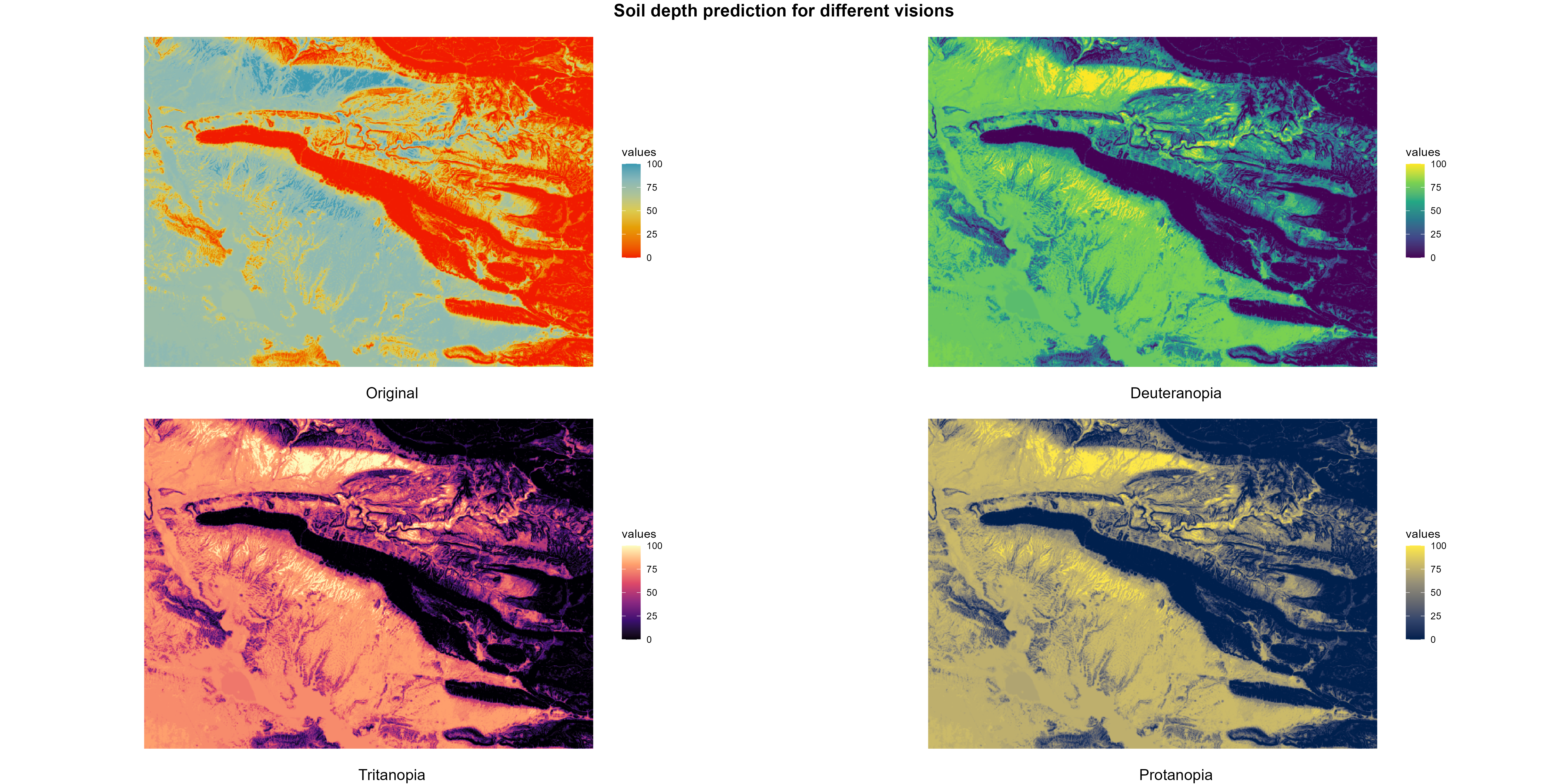
\(\\[0.5cm]\)
8.3.3 Export final maps
# 06.4 Final visualisations ====================================================
# Change parameters for uncertainty and predictions
soil_depth_visual <- c(predicted_raster_resize$median, predicted_raster_resize$uncertainty)
# Replace infinite values of the uncertainty with NA
soil_depth_visual$uncertainty[is.infinite(soil_depth_visual$uncertainty) & soil_depth_visual$uncertainty > 0] <- 9999
# Crop and mask
soil_depth_crop <- crop(soil_depth_visual, survey)
soil_depth_mask <- mask(soil_depth_visual, survey)
crs(soil_depth_mask) <- "EPSG:32638"
names(soil_depth_mask) <- c("Prediction", "Uncertainty")
rasterdf <- as.data.frame(soil_depth_mask, xy = TRUE)
rasterdf <- rasterdf[complete.cases(rasterdf),]
rasterdf$Uncertainty[rasterdf$Uncertainty == 9999] <- NA
bounds <- st_bbox(survey)
xlim_new <- c(bounds["xmin"] - 3000, bounds["xmax"] + 3000)
ylim_new <- c(bounds["ymin"] - 3000, bounds["ymax"] + 3000)
palette_wes <- rev(wes_palette("Zissou1", type = "continuous"))
palette_blue <- colorRampPalette(c("lightblue", "blue", "darkblue"))(7)
gg1 <- ggplot() +
geom_raster(data = rasterdf,
aes(x = x, y = y,fill = Prediction )) +
ggtitle("Soil depth prediction map") +
scale_fill_gradientn(colors = palette_wes,
name = "Soil depth (cm)") +
annotation_scale(
location = "br",
width_hint = 0.3,
height = unit(0.3, "cm"),
line_col = "black",
text_col = "black",
bar_cols = c("white", "red")
) +
annotate("text", label = paste("Projection: WGS84 UTM 38N"),
x = Inf, y = -Inf, hjust = 1.05, vjust = -3, size = 3, color = "black") +
annotation_north_arrow(location = "tr", which_north = "true", height = unit(1, "cm"), width = unit(0.75, "cm")) +
theme_bw() +
theme(
panel.grid = element_blank(),
axis.text.y = element_text(angle = 90, vjust = 0.5, hjust = 0.5),
axis.title = element_blank(),
legend.position = "right")+
coord_equal(ratio = 1)
gg1
ggsave("./export/Visualisation_soil_depth_prediction_maps.pdf", gg1, width = 20, height = 10)
ggsave("./export/Visualisation_soil_depth_prediction_maps.png", gg1, width = 20, height = 10)
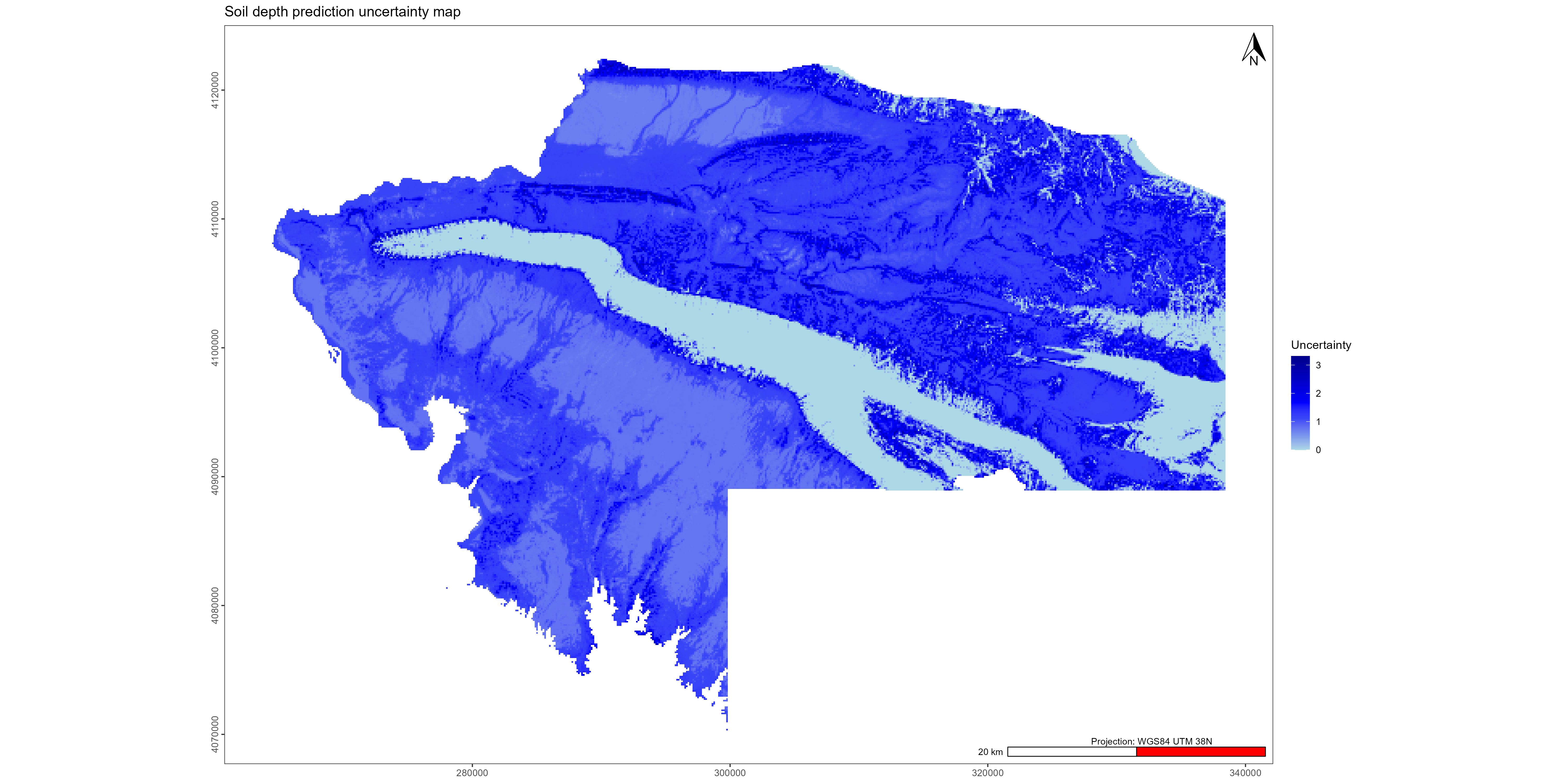
gg1 <- ggplot() +
geom_raster(data = rasterdf,
aes(x = x, y = y,fill = Uncertainty )) +
ggtitle("Soil depth uncertainty map") +
scale_fill_gradientn(colors = palette_blue,
name = "Uncertainty",
na.value = "lightgrey",
guide = guide_colorbar(order = 1)) +
new_scale_fill() +
geom_tile(data = data.frame(x = -Inf, y = -Inf, category = "NA"),
aes(x = x, y = y, fill = category), width = 0, height = 0) +
scale_fill_manual(name = "",values = c("NA" = "lightgrey"),guide = guide_legend(
override.aes = list(size = 3, shape = 22, fill = "lightgrey", color = "black"))) +
annotation_scale(
location = "br",
width_hint = 0.3,
height = unit(0.3, "cm"),
line_col = "black",
text_col = "black",
bar_cols = c("white", "red")
) +
annotate("text", label = paste("Projection: WGS84 UTM 38N"),
x = Inf, y = -Inf, hjust = 1.05, vjust = -3, size = 3, color = "black") +
annotation_north_arrow(location = "tr", which_north = "true", height = unit(1, "cm"), width = unit(0.75, "cm")) +
theme_bw() +
theme(
panel.grid = element_blank(),
axis.text.y = element_text(angle = 90, vjust = 0.5, hjust = 0.5),
axis.title = element_blank(),
legend.position = "right")+
coord_equal(ratio = 1)
gg1
ggsave("./export/Visualisation_soil_depth_uncertainty_prediction_maps.pdf", gg1, width = 20, height = 10)
ggsave("./export/Visualisation_soil_depth_uncertainty_prediction_maps.png", gg1, width = 20, height = 10)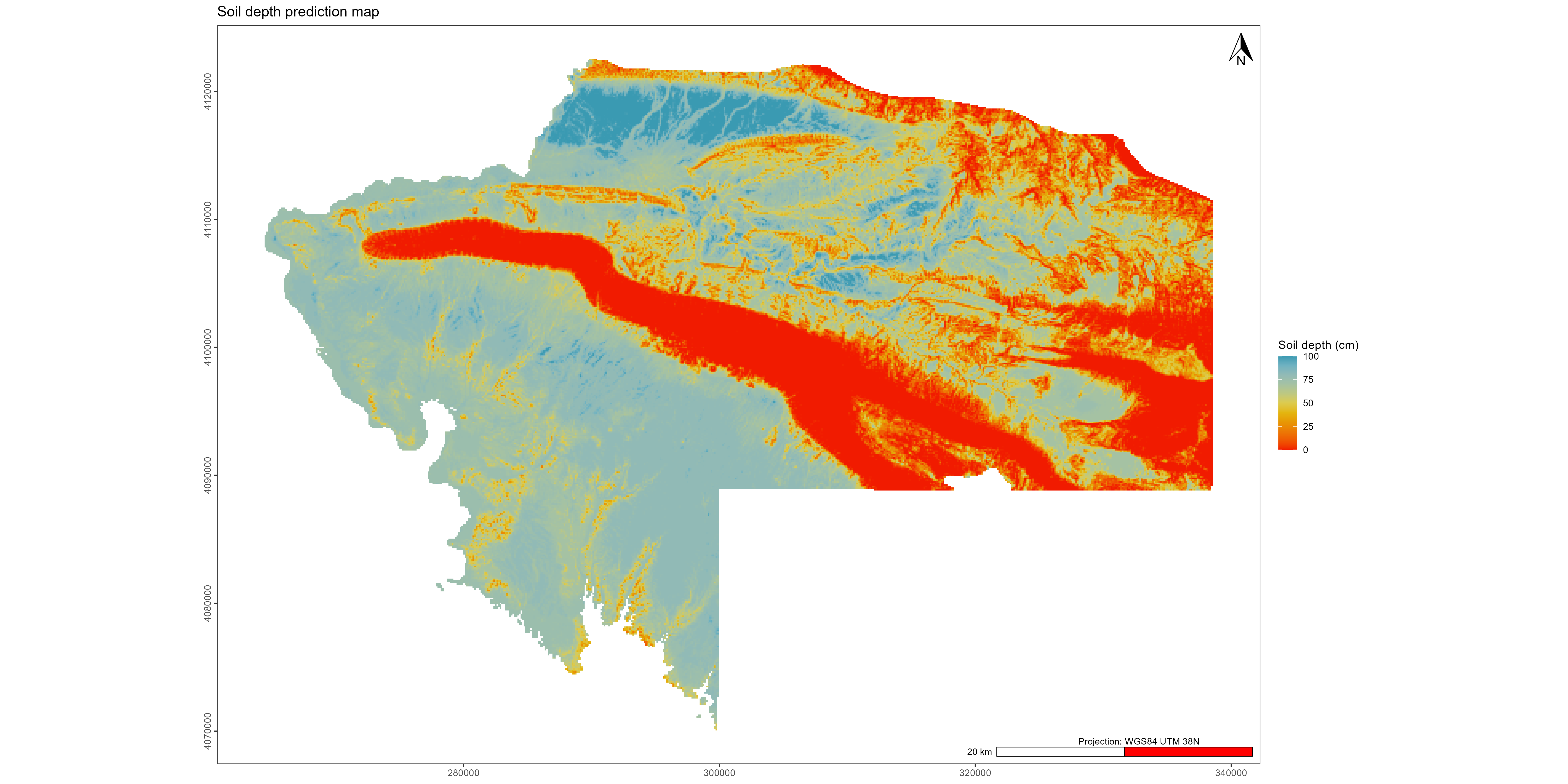
\(\\[0.5cm]\)
# 06.5 Simplified version for publication =======================================

gg1 <- ggplot() +
      geom_raster(data = rasterdf, aes(x = x, y = y, fill = Prediction)) +
      ggtitle("Soil depth prediction map") +
      scale_fill_gradientn(colors = palette_wes, name = "Soil depth in cm") +
      theme_void() +
      theme(
        legend.position = "right",
        plot.title = element_text(size = 8),
        legend.title = element_text(size = 10),
        legend.text = element_text(size = 8),
        legend.key.size = unit(0.7, "cm")) +
      coord_equal(ratio = 1)

gg2 <- ggplot() +
  geom_raster(data = rasterdf, aes(x = x, y = y, fill = Uncertainty)) +
  ggtitle("Soil depth uncertainty prediction map") +
  scale_fill_gradientn(colors = palette_blue, name = "Uncertainty", na.value = "lightgrey",
                       guide = guide_colorbar(order = 1)) +

  new_scale_fill() +
  geom_tile(data = data.frame(x = -Inf, y = -Inf, category = "NA"),
            aes(x = x, y = y, fill = category), width = 0, height = 0) +

  scale_fill_manual(name = "",values = c("NA" = "lightgrey"),guide = guide_legend(
    override.aes = list(size = 3, shape = 22, fill = "lightgrey", color = "black"))) +


  theme_void() +
  theme(
    legend.position = "right",
    plot.title = element_text(size = 8),
    legend.title = element_text(size = 10),
    legend.text = element_text(size = 8),
    legend.key.size = unit(0.7, "cm")) +
  coord_equal(ratio = 1)

combined_plot <- plot_grid(gg1, gg2, ncol = 2)

plot(combined_plot)

ggsave("./export/Publication_soil_depth_map.pdf", combined_plot, width = 20, height = 10)
ggsave("./export/Publication_soil_depth_map.png", combined_plot, width = 20, height = 10)

dev.off()