6 Spectra model prediction
We used only the raw spectra and three spectra transformations from the 15 spectra produced in the FTIR part. This transformation are improving the quality of the prediction model (Ludwig et al. 2023). In total we had four spectra:
- Raw spectra.
- SG-2-11 the Savitzky-Golay with a polynomial order of 2 and a window size of 11.
- Moving average of 11. -SNV-SG standard normal variate transformation on the Savitzky-Golay with a polynomial order of 2 and a window size of 11.
6.1 Model implementation
We implemented the prediction model in Python language. A sanity check was performed to assess the conformity of the data set Sanity_Check_code.
We split the data into an 85% training set and a 15% testing set.
As EC values had outliers we removed all samples with values higher than 400 µS/cm: 53802 (827 µS/cm), 53871 (857 µS/cm), 53872 (932 µS/cm), 53902 (718 µS/cm), 53938 (447 µS/cm), 53954 (426 µS/cm) and 55852 (636 µS/cm).
All the properties were predicted using the Cubist model under Python environment Cubist_Kfold_code. A 5 time stratified k-fold was used with a total of 9 combinations for the hyperparameter. The stratified k-fold helps have a higher diversity of sampling in the training and testing set.
| n_rules | n_committees |
|---|---|
| 20 | 5 |
| 30 | 5 |
| 40 | 5 |
| 20 | 10 |
| 30 | 10 |
| 40 | 10 |
| 20 | 15 |
| 30 | 15 |
| 40 | 15 |
6.2 Model evaluation
6.2.1 All spectra tranformations metrics
| Metric | ME | R2 | RMSE | RPIQ |
|---|---|---|---|---|
| pH | -0.1130862 | 0.4401298 | 0.1479898 | 1.2423942 |
| CaCO3 | -1.3252205 | 0.8882458 | 4.1193275 | 2.3192395 |
| Nt | -0.0210327 | 0.6229612 | 0.0543926 | 1.4595850 |
| Ct | -0.2208946 | 0.8913525 | 0.5595367 | 2.3885632 |
| OC | -0.0612059 | 0.5264148 | 0.6699846 | 0.9218613 |
| EC | -30.6617828 | 0.1141583 | 66.3535662 | 0.9523699 |
| Sand | -6.3994920 | 0.7674734 | 7.3599863 | 2.3624346 |
| Silt | 3.2742514 | 0.2136148 | 9.3070178 | 0.8782774 |
| Clay | 3.5598760 | 0.6930271 | 7.9695160 | 2.3912120 |
| MWD | -0.0183279 | 0.4745772 | 0.0539841 | 1.2472350 |
\[\\[1.5cm]\]
| Metric | ME | R2 | RMSE | RPIQ |
|---|---|---|---|---|
| pH | -0.0822356 | 0.4621653 | 0.1450483 | 1.221859 |
| CaCO3 | -0.0115416 | 0.8820737 | 4.2315510 | 2.389729 |
| Nt | -0.0207909 | 0.6334873 | 0.0536280 | 1.410630 |
| Ct | -0.0333944 | 0.9101929 | 0.5087145 | 2.228431 |
| OC | -0.0276244 | 0.5112682 | 0.6806143 | 1.087405 |
| EC | -16.8330812 | 0.1914366 | 63.3932824 | 1.114983 |
| Sand | -6.9387918 | 0.7336180 | 7.8775860 | 2.300951 |
| Silt | 0.4148447 | 0.1086026 | 9.9089712 | 0.875066 |
| Clay | 6.7544251 | 0.7609876 | 7.0322156 | 2.343124 |
| MWD | -0.0284105 | 0.4724332 | 0.0540942 | 1.331620 |
\[\\[1.5cm]\]
| Metric | ME | R2 | RMSE | RPIQ |
|---|---|---|---|---|
| pH | 0.0139322 | 0.4081296 | 0.1521604 | 0.9712110 |
| CaCO3 | -0.0466458 | 0.9012224 | 3.8727870 | 2.7690478 |
| Nt | 0.0136756 | 0.3532399 | 0.0712392 | 0.4787131 |
| Ct | -0.0795040 | 0.8415988 | 0.6756130 | 1.8099295 |
| OC | -0.0751953 | 0.2343362 | 0.8518925 | 0.3591207 |
| EC | 37.7198879 | 0.0463005 | 68.8481029 | 0.9539687 |
| Sand | -2.6170488 | 0.7616948 | 7.4508777 | 2.4868337 |
| Silt | -4.7215761 | 0.3247059 | 8.6246080 | 0.9129198 |
| Clay | -3.5665841 | 0.7175530 | 7.6445239 | 2.4276119 |
| MWD | 0.0299509 | 0.4394541 | 0.0557593 | 1.1867736 |
\[\\[1.5cm]\]
| Metric | ME | R2 | RMSE | RPIQ |
|---|---|---|---|---|
| pH | -0.1487360 | 0.3990151 | 0.1533275 | 0.8891613 |
| CaCO3 | -1.1519722 | 0.8888660 | 4.1078803 | 2.7618729 |
| Nt | -0.0046014 | 0.8257789 | 0.0369741 | 1.7119021 |
| Ct | 0.0367057 | 0.9123964 | 0.5024348 | 2.7212452 |
| OC | 0.1736385 | 0.6126784 | 0.6059009 | 1.1525632 |
| EC | -5.9358389 | 0.2942953 | 59.2239976 | 0.9349021 |
| Sand | 2.0420108 | 0.8106039 | 6.6424182 | 2.6565763 |
| Silt | 0.1929490 | 0.3783928 | 8.2746742 | 0.9772474 |
| Clay | -1.7827777 | 0.6928479 | 7.9718426 | 2.2699483 |
| MWD | -0.0022866 | 0.4592173 | 0.0547675 | 1.1640412 |
6.2.2 Selected transformed spectra
Regarding the results of the predictions, we selected for each variables the following spectra:
- pH Raw spectra.
- CaCO\(_3\) SG.2.11 spectra.
- Nt SNV-SG spectra.
- Ct SNV-SG spectra.
- OC SNV-SG spectra.
- EC SNV-SG spectra.
- Sand SNV-SG spectra.
- Silt SNV-SG spectra.
- Clay SG.2.11 spectra.
- MWD Raw spectra.
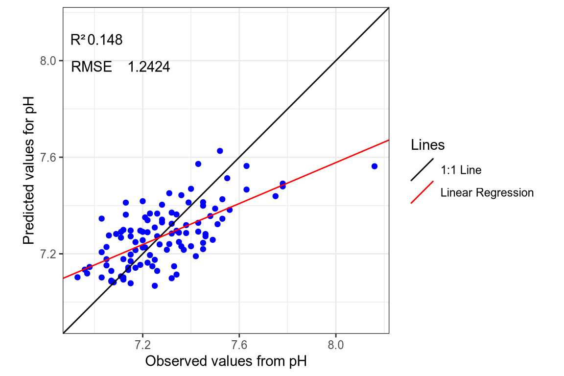
(#fig:regression plot 1)Regression curve of the predicted pH values.
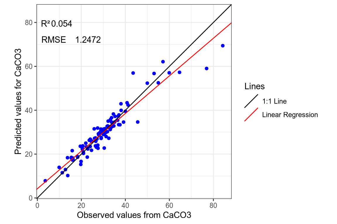
(#fig:regression plot 2)Regression curve of the predicted CaCo3 values.
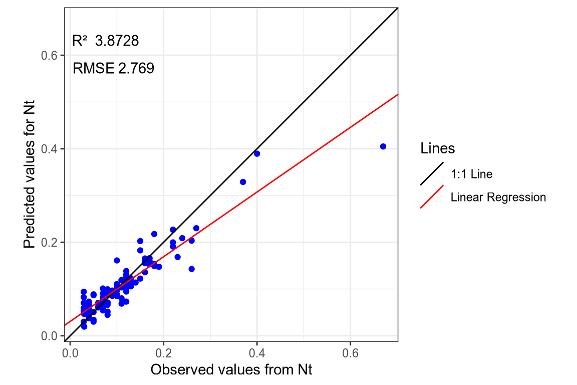
(#fig:regression plot 3)Regression curve of the predicted Nt values.
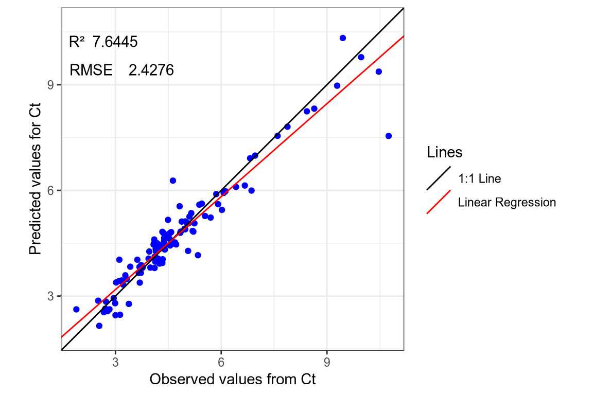
(#fig:regression plot 4)Regression curve of the predicted Ct values.
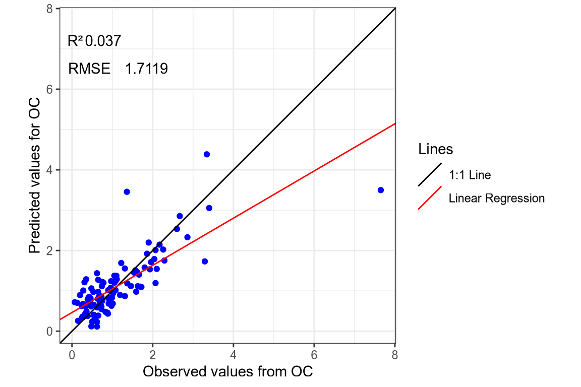
(#fig:regression plot 5)Regression curve of the predicted SOC values.
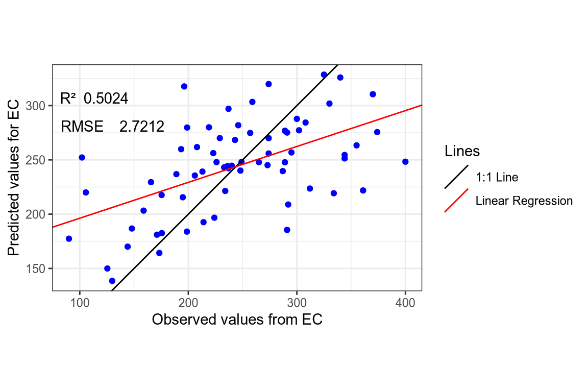
(#fig:regression plot 6)Regression curve of the predicted EC values.
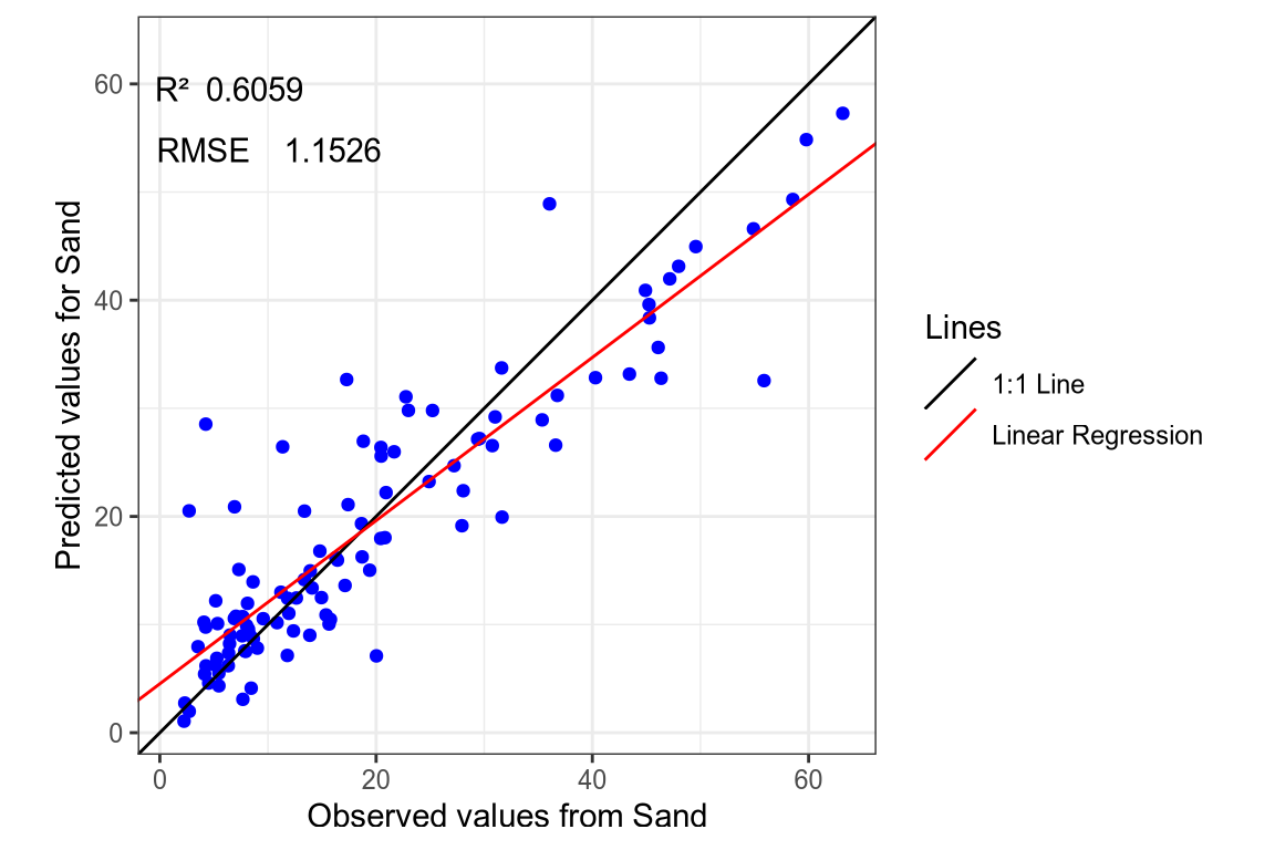
(#fig:regression plot 7)Regression curve of the predicted Sand values.
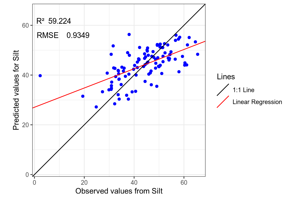
(#fig:regression plot 8)Regression curve of the predicted Silt values.
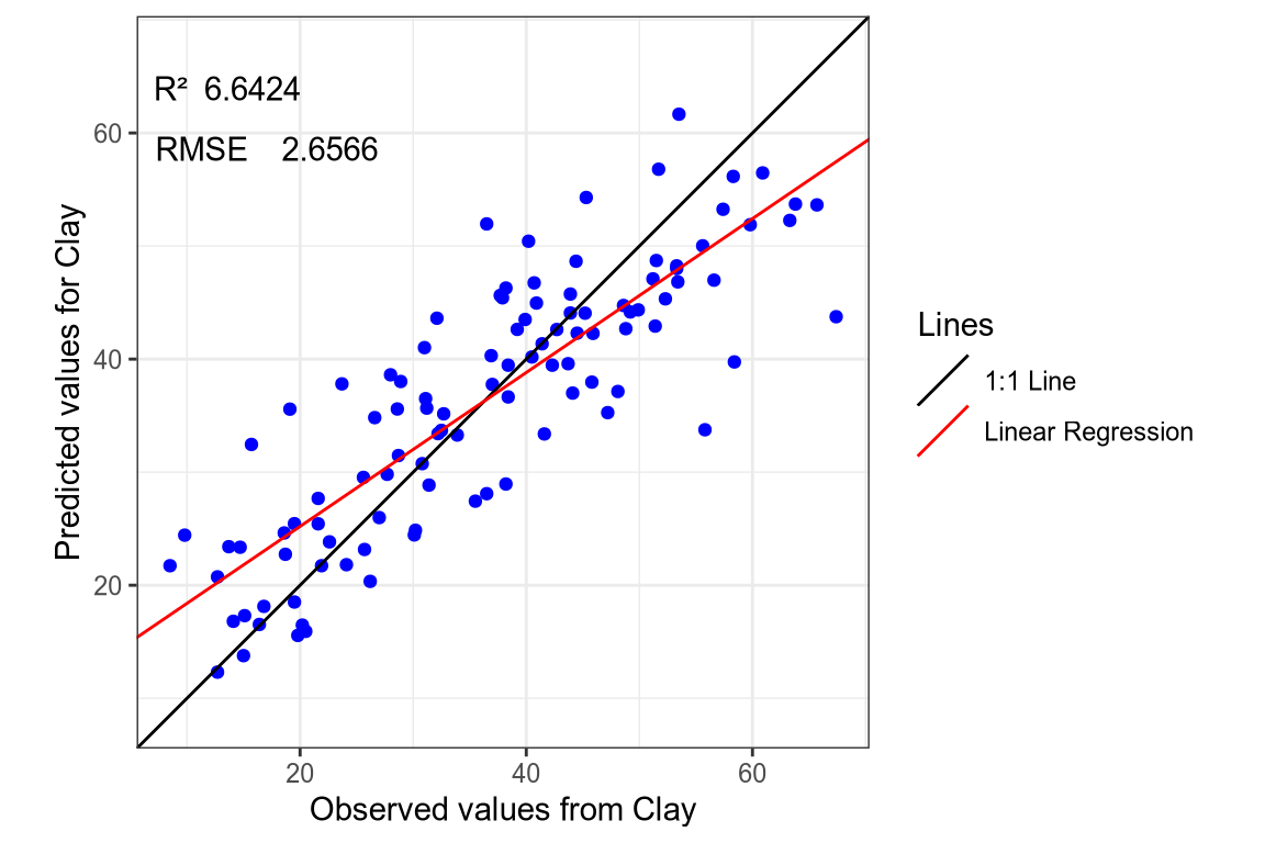
(#fig:regression plot 9)Regression curve of the predicted Clay values.
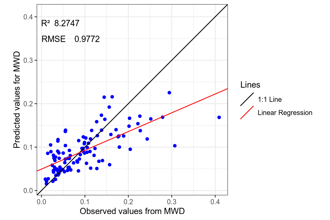
(#fig:regression plot 10)Regression curve of the predicted MWD values.
6.3 Predicted values
6.3.1 Full predicted values table
The full table of 2022 and 2023 samples predicted is visible below or can be found on the deposit as Mir_spectra_prediction file or at: https://doi.org/10.1594/PANGAEA.973700.
## Rows: 532 Columns: 18
## ── Column specification ───────────────────────────────────────
## Delimiter: ";"
## chr (1): Event label
## dbl (16): Lab label, Latitude, Longitude, Depth, top, Depth, bot, Weight, p...
## dttm (1): Date
##
## ℹ Use `spec()` to retrieve the full column specification for this data.
## ℹ Specify the column types or set `show_col_types = FALSE` to quiet this message.We removed the sample with ID 55864 which is an outlier.
6.3.2 Boxplot of the predicted values
# Component values ======================================
par(mfrow = c(2, 5), mar = c(3.1, 2.1, 1.1, .1), oma = c(0, 2.5, 2, 5.9),
mgp = c(1.8, 0.6, 0), las = 0, cex.lab = 1, cex.axis = 1, xpd = FALSE)
# c(min(Soil_Data_Observed$pH)-0.1, max(Soil_Data_Observed$pH)+0.1))
boxplot(Prediction$pH, xlab = "pH", ylab = "", ylim = c(min(Prediction$pH)-0.1, max(Prediction$pH)+0.1))
boxplot(Prediction$CaCO3, xlab = expression("CaCO"[3]), ylab = "", ylim = c(0,100)); title(ylab = "%", line = 2.25)
boxplot(Prediction$Nt, xlab = "Nt", ylab = "", ylim = c(0, 0.3)); title(ylab = "%", line = 2.25)
boxplot(Prediction$Ct, xlab = "Ct", ylab = "", ylim = c(0,15)); title(ylab = "%", line = 2.25)
boxplot(Prediction$OC, xlab = "OC", ylab = "", ylim = c(0, 4.1)); title(ylab = "%", line = 2.25)
boxplot(Prediction$EC, xlab = "EC", ylab = "", ylim = c(150, 350)); title(ylab = "µS/cm", line = 2.25)
boxplot(Prediction$Sand, xlab = "Sand", ylab = "", ylim = c(0, 100)); title(ylab = "%", line = 2.25)
boxplot(Prediction$Silt, xlab = "Silt", ylab = "", ylim = c(0, 100)); title(ylab = "%", line = 2.25)
boxplot(Prediction$Clay, xlab = "Clay", ylab = "", ylim = c(0, 100)); title(ylab = "%", line = 2.25)
boxplot(Prediction$MWD, xlab = "MWD", ylab = "", ylim = c(0, 0.25)); title(ylab = "mm", line = 2.25)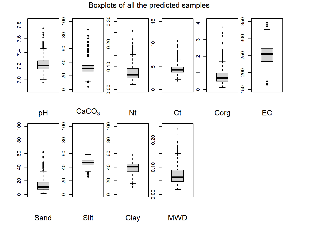
(#fig:plot boxplot full)Boxplots of all the predicted samples.
\[\\[1.5cm]\]
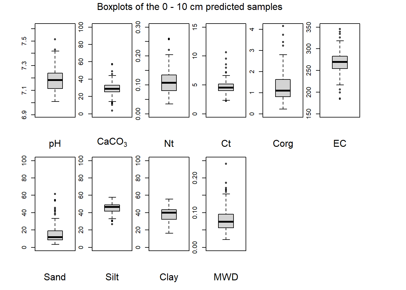
(#fig:plot boxplot zero-ten)Boxplots of the 0 - 10 cm predicted samples.
\[\\[1.5cm]\]
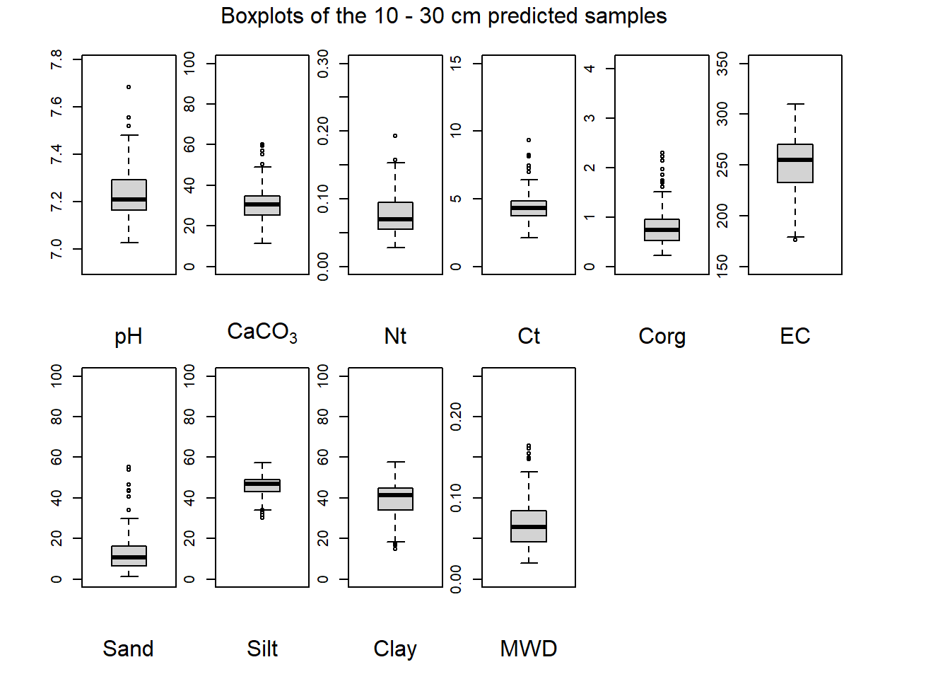
(#fig:plot boxplot ten-thirty)Boxplots of the 10 - 30 cm predicted samples.
\[\\[1.5cm]\]
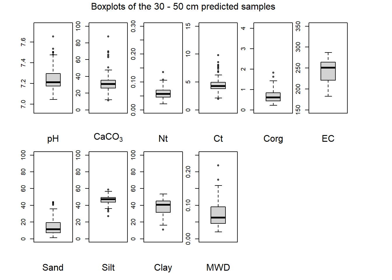
(#fig:plot boxplot thirty-fifty)Boxplots of the 30 - 50 cm predicted samples.
\[\\[1.5cm]\]
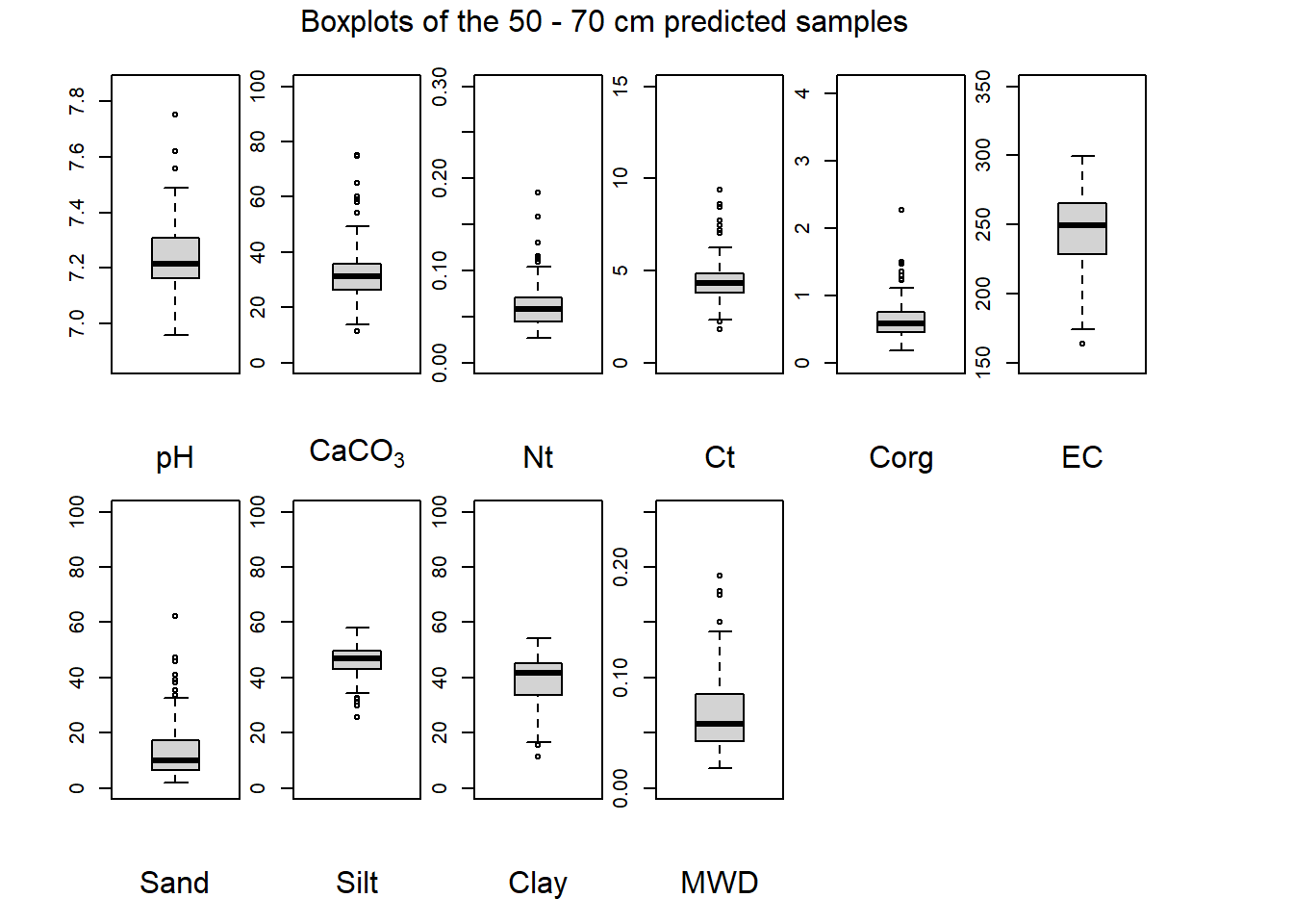
(#fig:plot boxplot fifty-seventy)Boxplots of the 50 - 70 cm predicted samples.
\[\\[1.5cm]\]
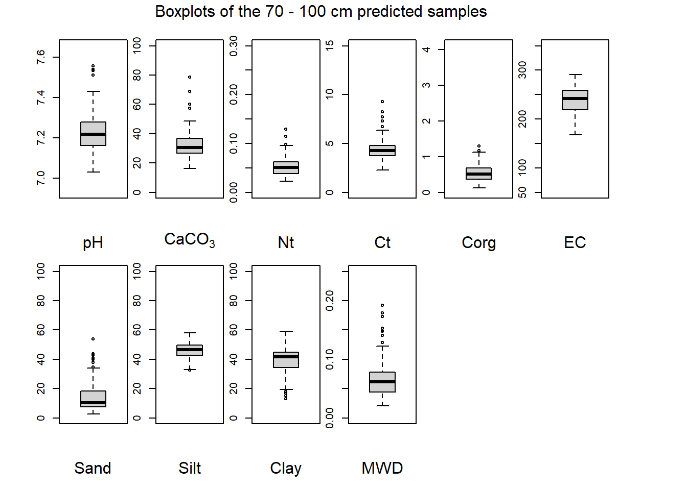
(#fig:plot boxplot seventy-hundred)Boxplots of the 70 - 100 cm predicted samples.
6.3.3 Texture of the predicted samples
We ploted the soil texture according to (WRB 2006) classification.
#Soil texture
texture <- data.frame("SAND" = Prediction$Sand, "SILT" = Prediction$Silt, "CLAY" = Prediction$Clay)
row.names(texture) <- Prediction$`Lab label`
texture <- na.omit(texture)
texture_resize <- texture[,c(1:3)]
texture_resize <- TT.normalise.sum(texture_resize, css.names = c("SAND","SILT", "CLAY"))
texture_resize <- TT.text.transf(
tri.data = texture_resize, dat.css.ps.lim = c(0, 0.002, 0.063, 2), # German system
base.css.ps.lim = c(0, 0.002, 0.05, 2) # USDA system
)TT.plot(class.sys = "USDA.TT", tri.data = texture_resize, main = "", frame.bg.col = "#f2f2f2", grid.show = FALSE, arrows.show = TRUE, col = "#c96dc4", pch = 19, cex.axis = 0.9, cex = 0.3, lwd.lab = 1.2, lwd.axis = 1.5, cex.lab = 1.4, new.mar = c(5, 0, 1, 0), css.lab = c("Clay", "Silt", "Sand"))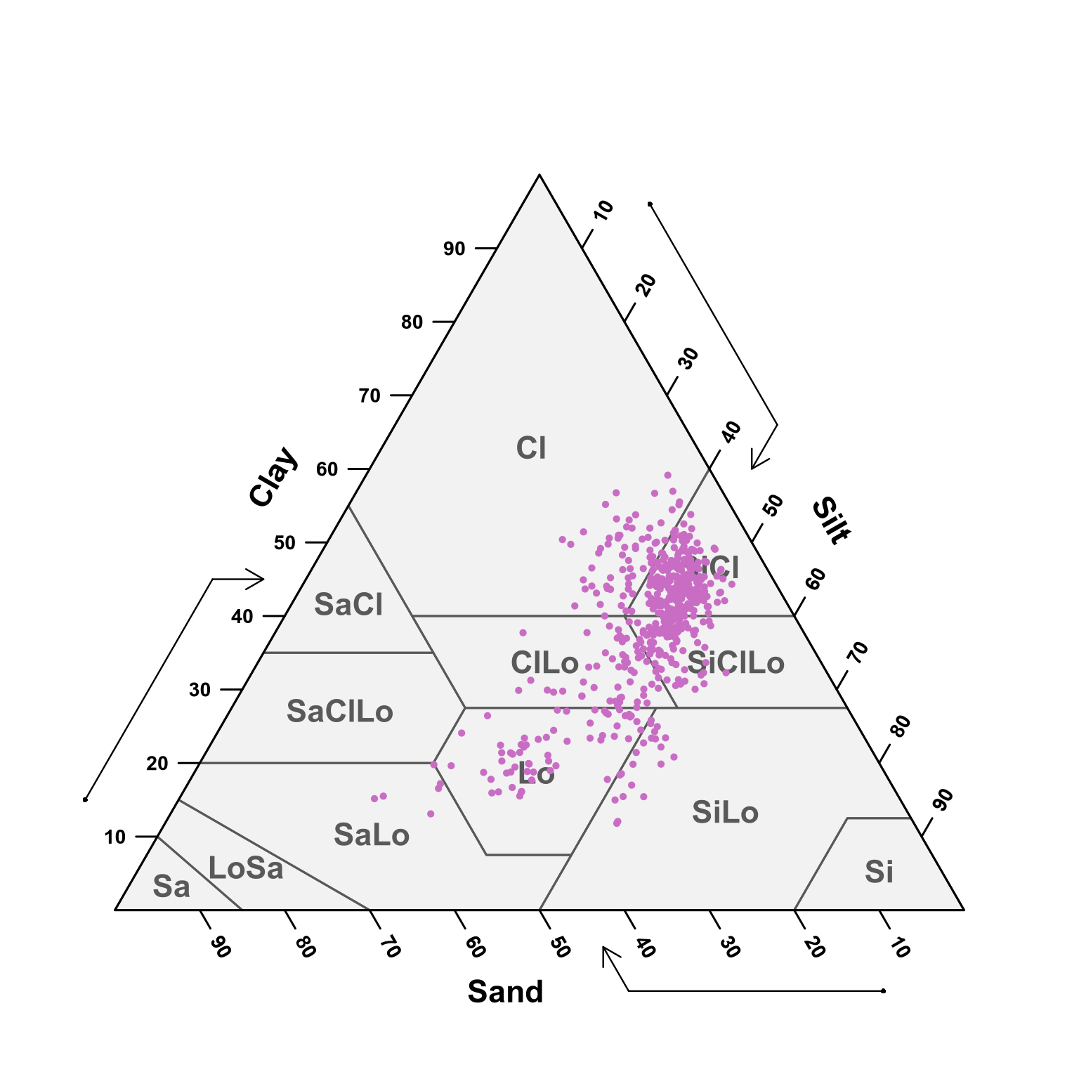
(#fig:soil ploting pred)USDA texture of the predicted samples for all depths.
#Soil texture
texture <- data.frame("SAND" = Prediction$Sand, "SILT" = Prediction$Silt, "CLAY" = Prediction$Clay, "depth" = Prediction$`Depth, bot`)
row.names(texture) <- Prediction$`Lab label`
texture <- na.omit(texture)
texture_resize <- texture[,c(1:3)]
texture_resize <- TT.normalise.sum(texture_resize, css.names = c("SAND","SILT", "CLAY"))
texture_resize <- TT.text.transf(
tri.data = texture_resize, dat.css.ps.lim = c(0, 0.002, 0.063, 2), # German system
base.css.ps.lim = c(0, 0.002, 0.05, 2) # USDA system
)
texture <- cbind(texture_resize, texture[,4])
text.zero <- texture[texture[,4] == 0.1,]
text.ten <- texture[texture[,4] == 0.3,]
text.thirty <- texture[texture[,4] == 0.5,]
text.fifty <- texture[texture[,4] == 0.7,]
text.seventy <- texture[texture[,4] == 1,]\[\\[1.5cm]\]
TT.plot(class.sys = "USDA.TT", tri.data = text.zero, main = "", frame.bg.col = "#f2f2f2", grid.show = FALSE, arrows.show = TRUE, col = "#c96dc4", pch = 19, cex.axis = 0.9, cex = 0.3, lwd.lab = 1.2, lwd.axis = 1.5, cex.lab = 1.4, new.mar = c(5, 0, 1, 0), css.lab = c("Clay", "Silt", "Sand"))
(#fig:soil depth zero - ten ploting pred)USDA texture of the predicted samples for 0 - 10 cm samples.
\[\\[1.5cm]\]

(#fig:soil depth ten-thirty ploting pred)USDA texture of the predicted samples for 10 - 30 cm samples.
\[\\[1.5cm]\]

(#fig:soil depth thirty-fifty ploting pred)USDA texture of the predicted samples for 30 - 50 cm samples.
\[\\[1.5cm]\]
(#fig:soil depth fifty-seventy ploting pred)USDA texture of the predicted samples for 50 - 70 cm samples.
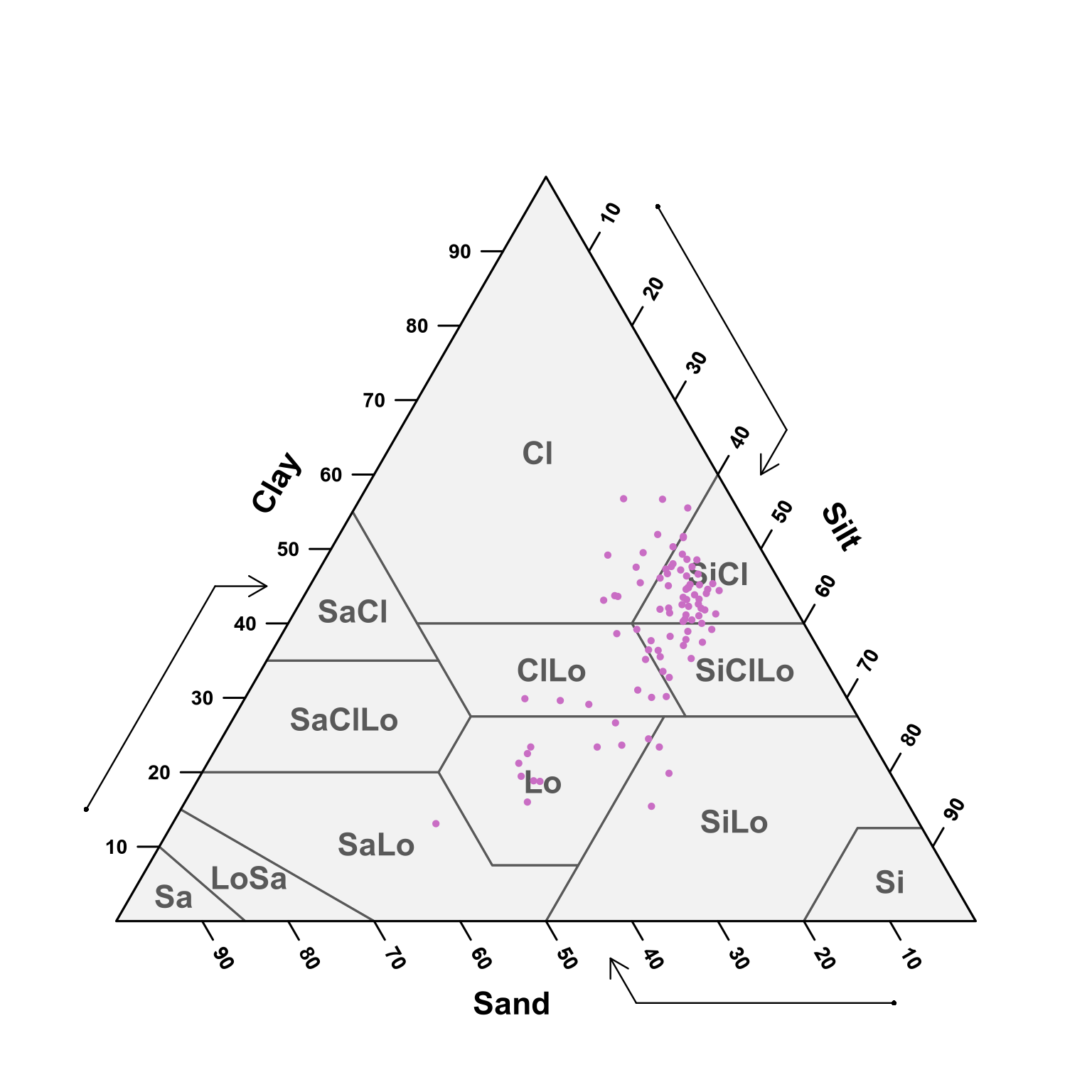
\[\\[1.5cm]\]
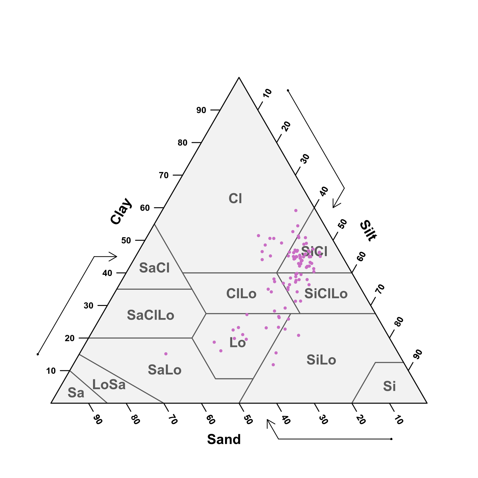
(#fig:soil depth weventy-hundred ploting pred)USDA texture of the predicted samples for 70 - 100 cm samples.
6.4 Observed vs. predicted values
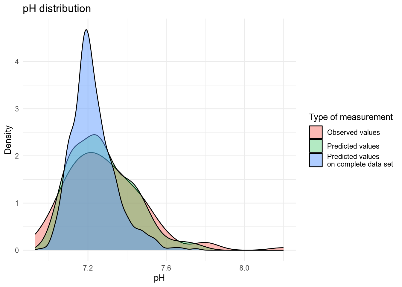
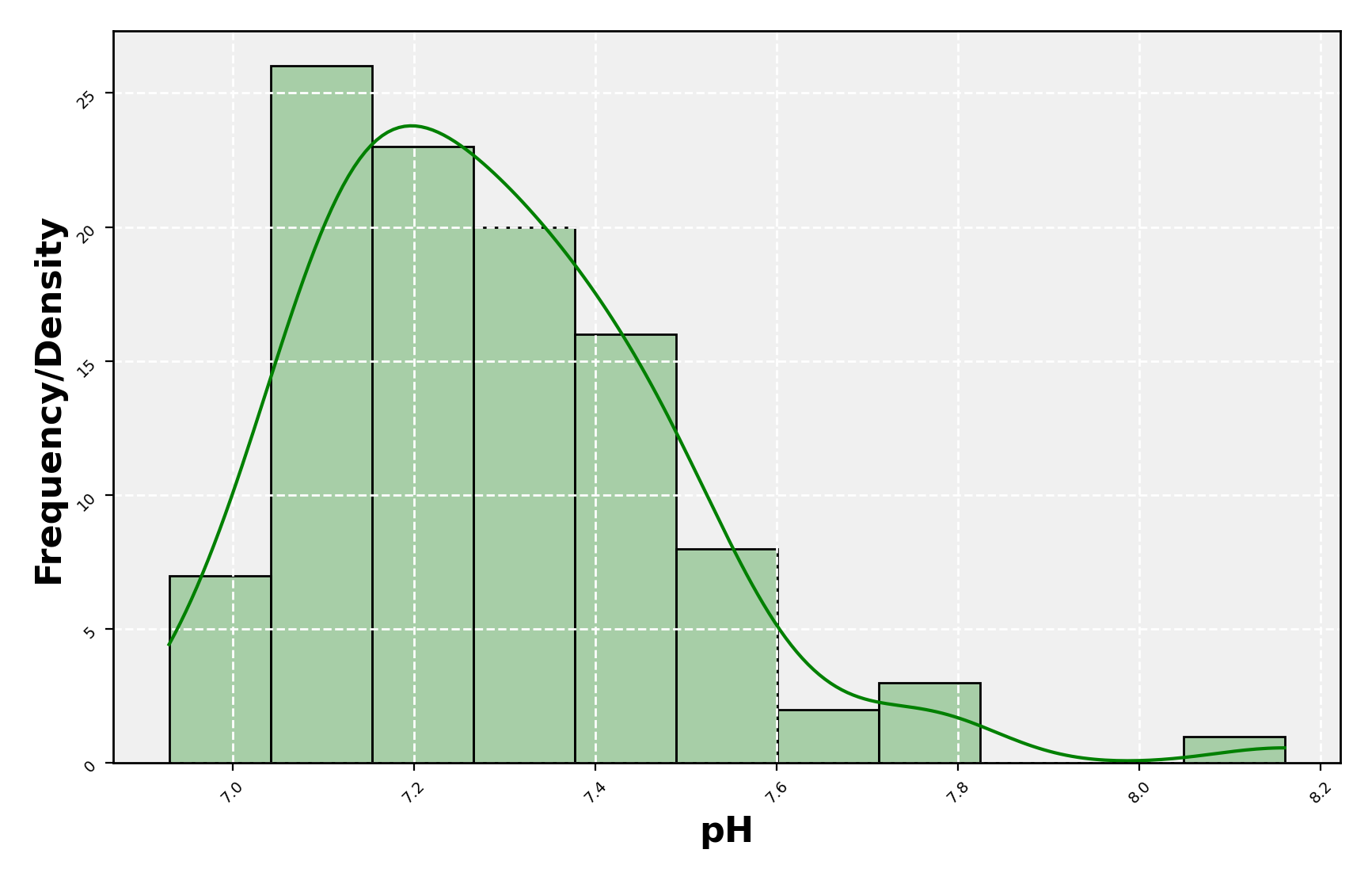
(#fig:density plot predicted 1)Density plot of pH values.
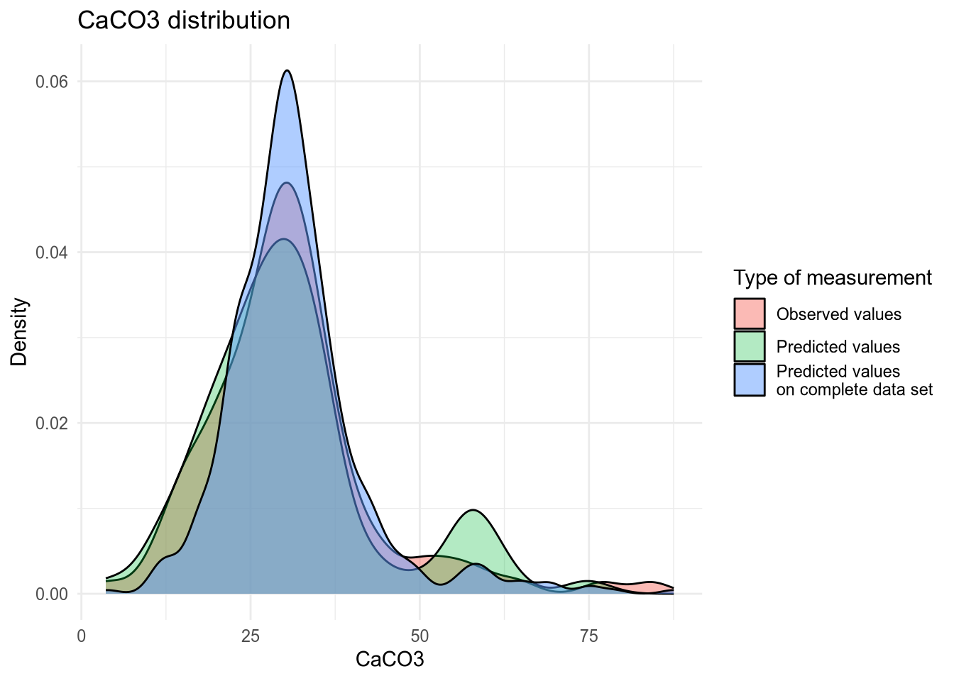
(#fig:density plot predicted 2)Density plot of CaC03 values.
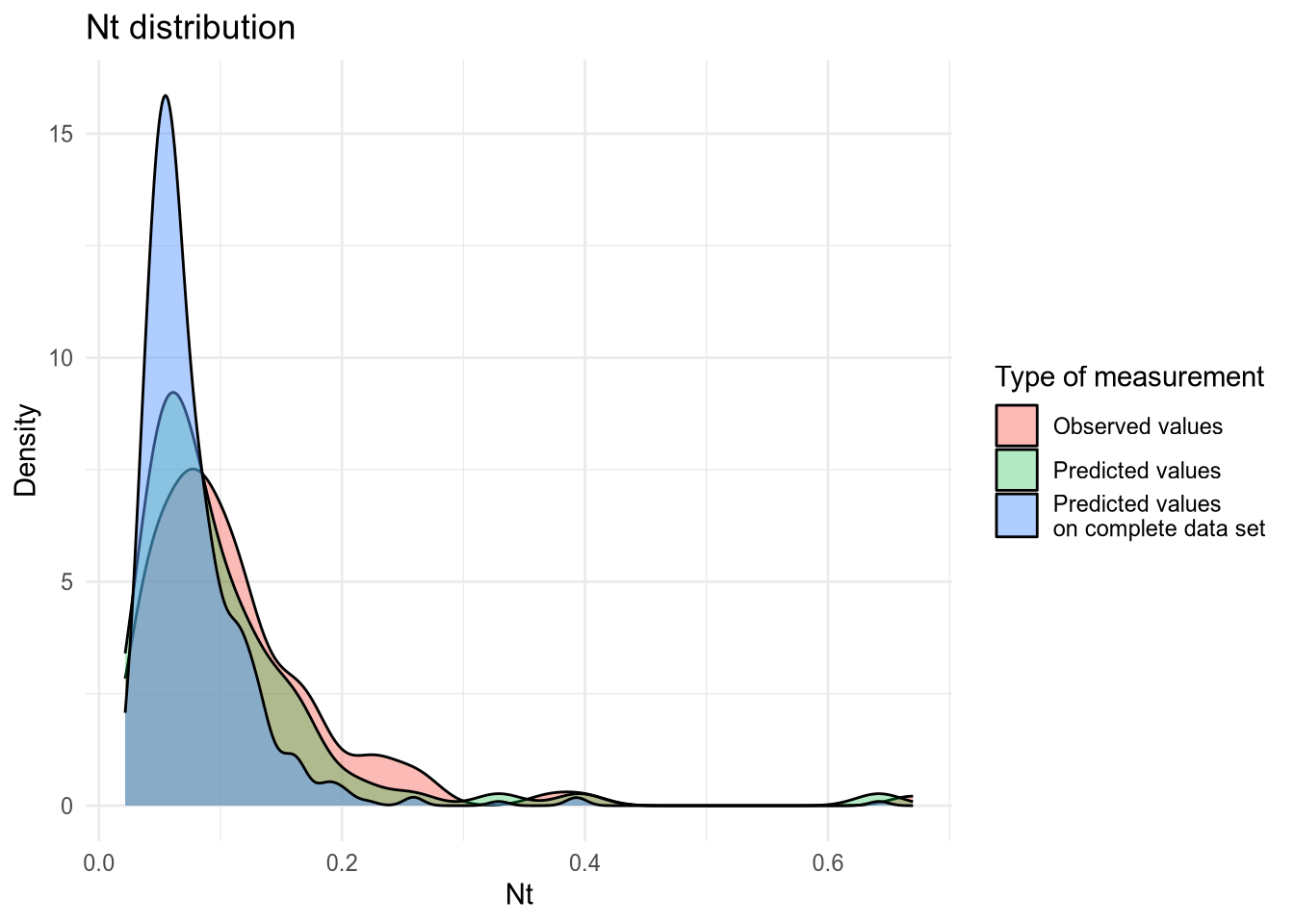
(#fig:density plot predicted 3)Density plot of Nt values.
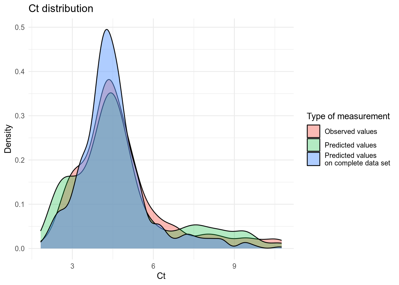
(#fig:density plot predicted 4)Density plot of Ct values.
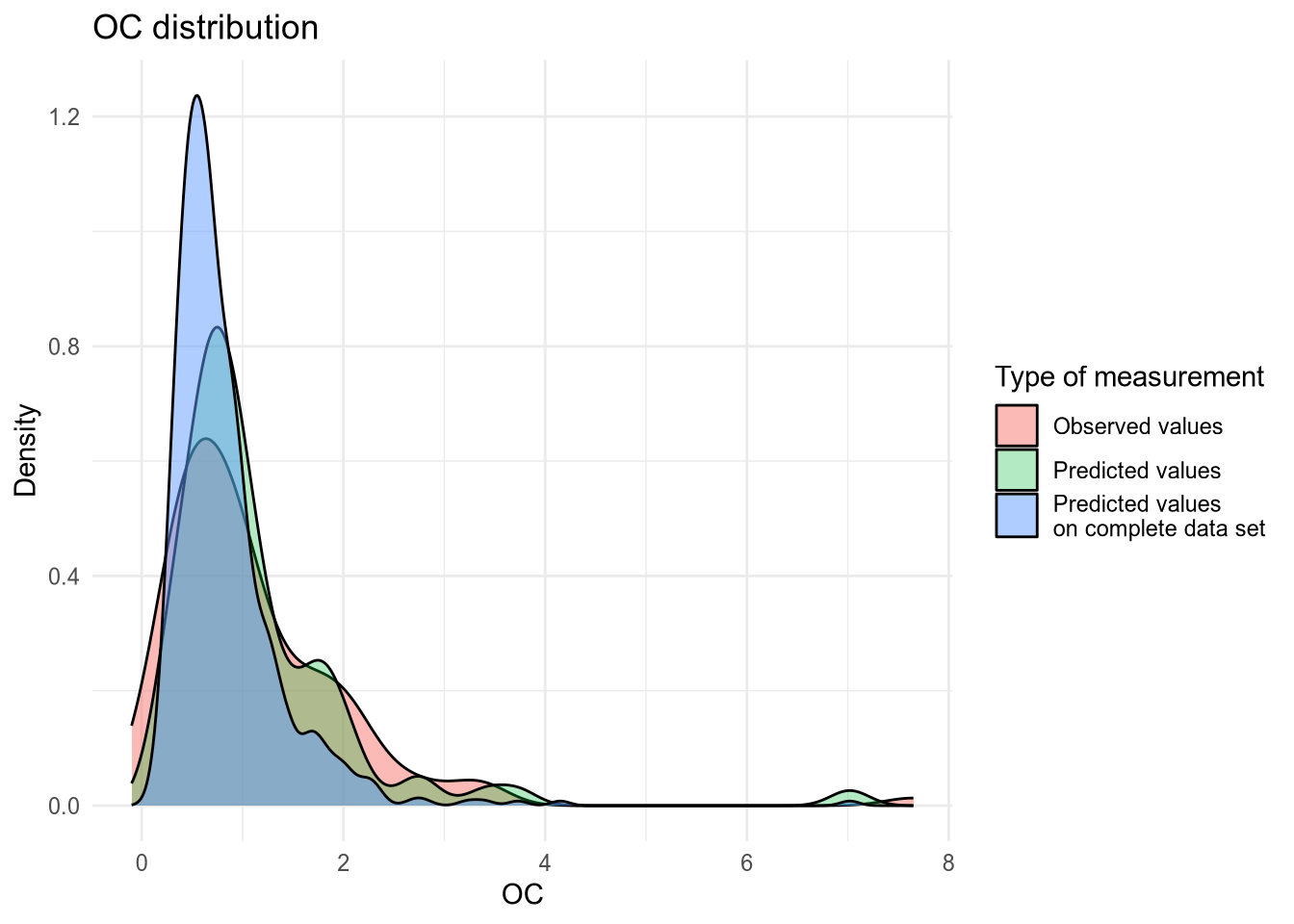
(#fig:density plot predicted 5)Density plot of OC values.
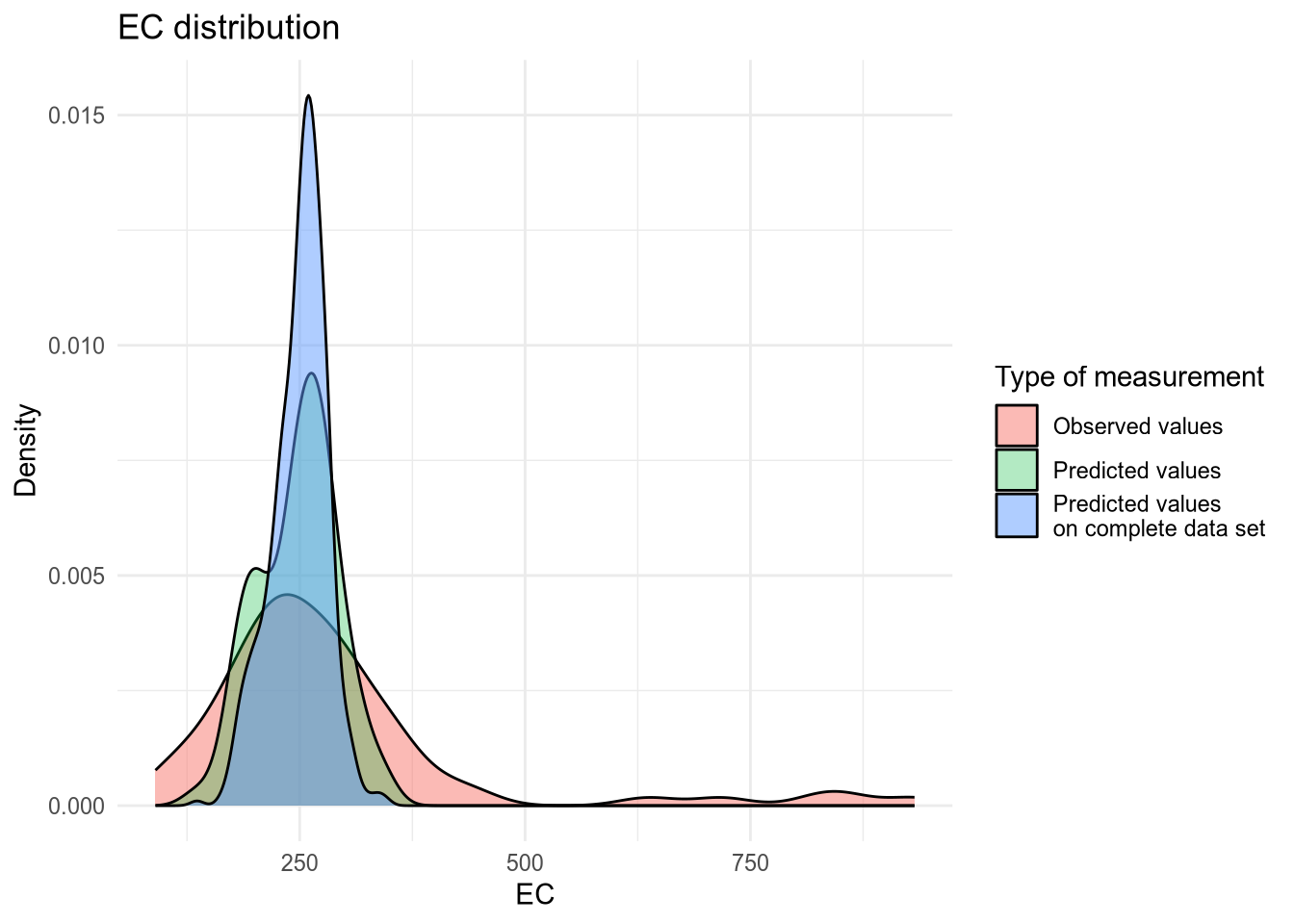
(#fig:density plot predicted 6)Density plot of EC values.
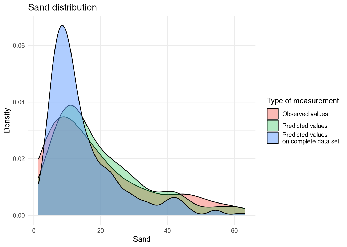
(#fig:density plot predicted 7)Density plot of Sand values.
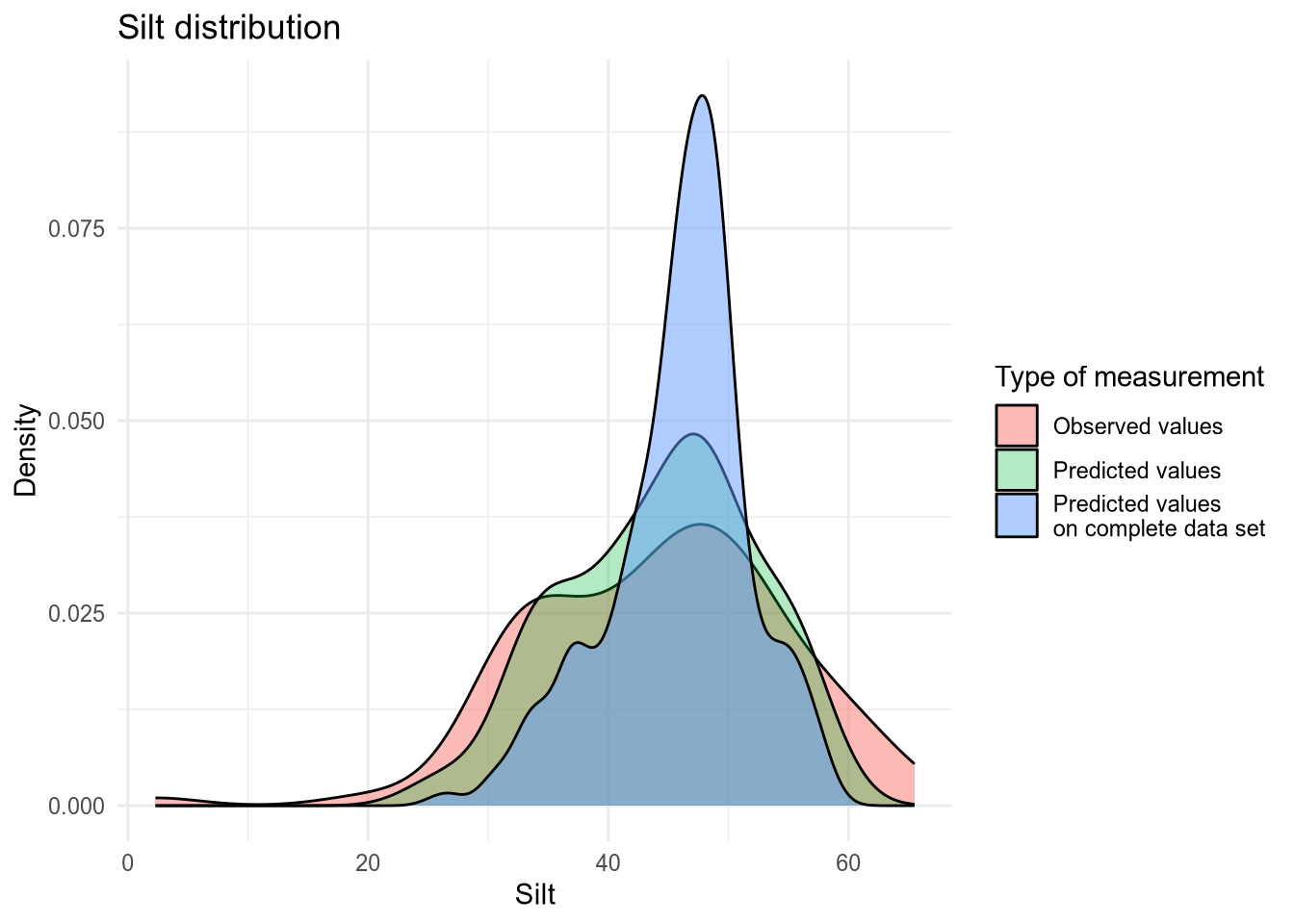
(#fig:density plot predicted 8)Density plot of Silt values.
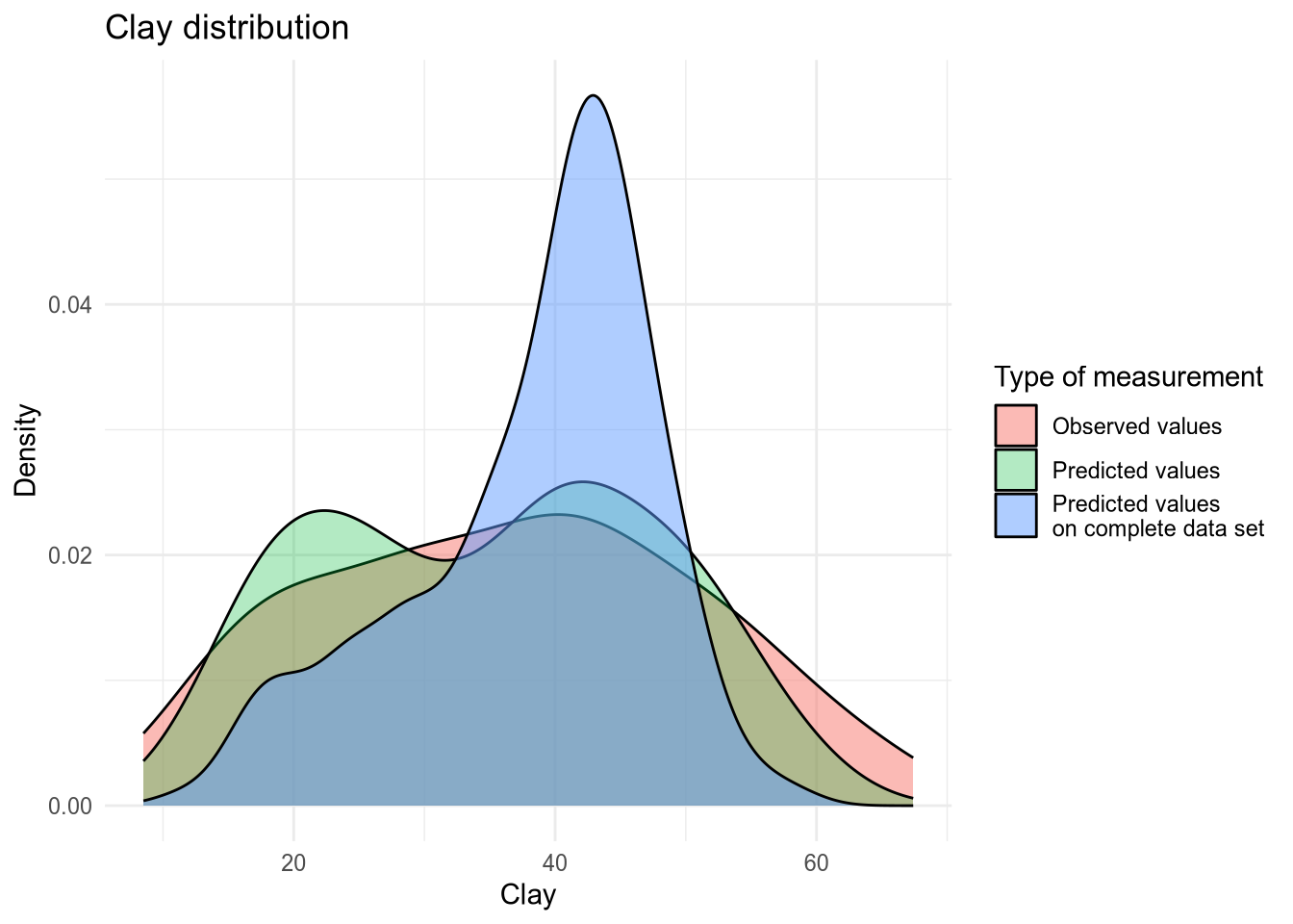
(#fig:density plot predicted 9)Density plot of Clay values.
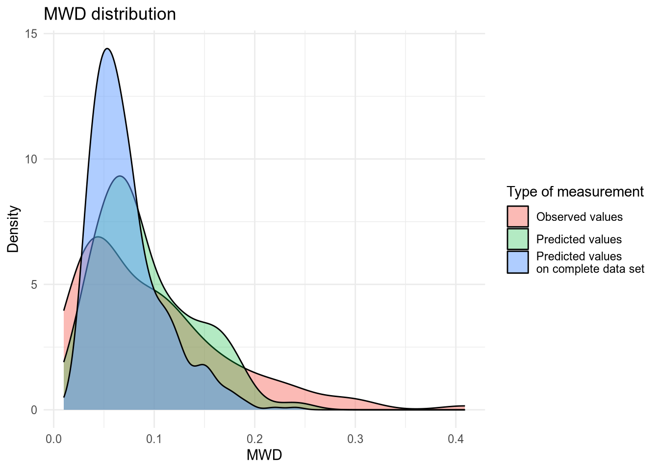
(#fig:density plot predicted 10)Density plot of MWD values.